Measurements conducted 19.-21.7.2013.
Optical and structural properties of raspberry leaves (and a small sample of fireweed).
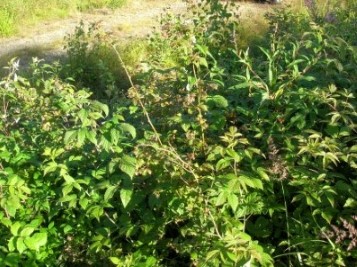
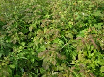
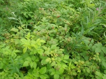
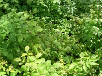
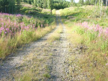
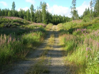
4.1 Sample locations
Four (4) locations of raspberry, and
three (3) of fireweed were selected. The stand was the same as used for
collecting specific leaf area samples in 1).
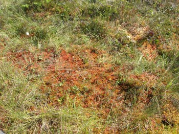
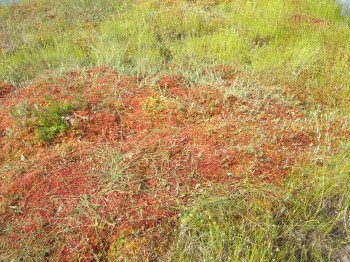
Selected fresh-looking, green canopies. The leaves were already yellowish in most parts of the stand due to the dry season.
Shoots (1-3) from each location were cut and brought to the laboratory. For raspberry, separate samples of 1st year and 2nd year shoots were selected.
While waiting for the measurements, the shoots were kept in a cooling room (7 ºC), in a bucket of water, the lights on.
The maximum time between cutting the shoots and making the measurement was ~4 hours.
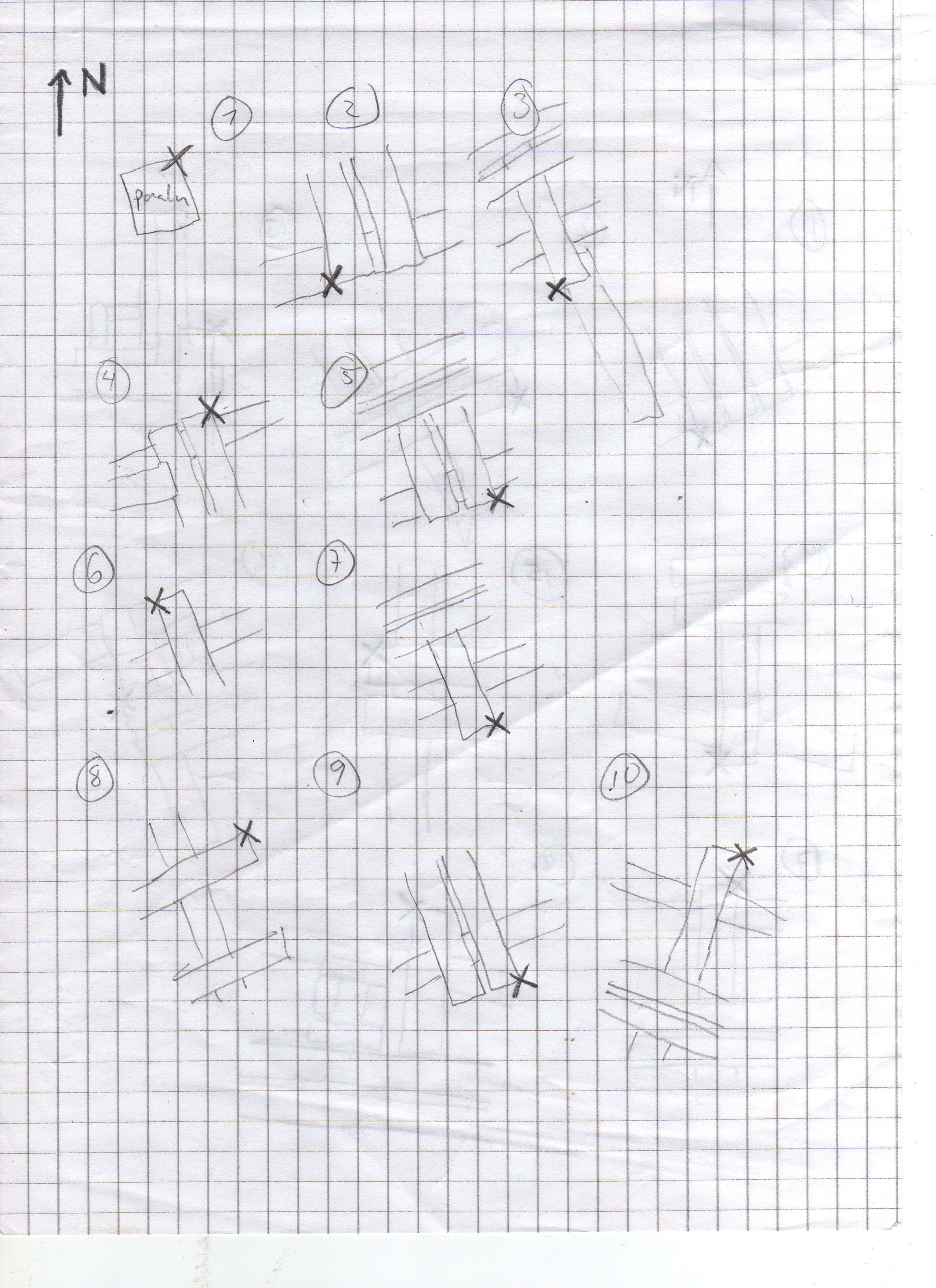
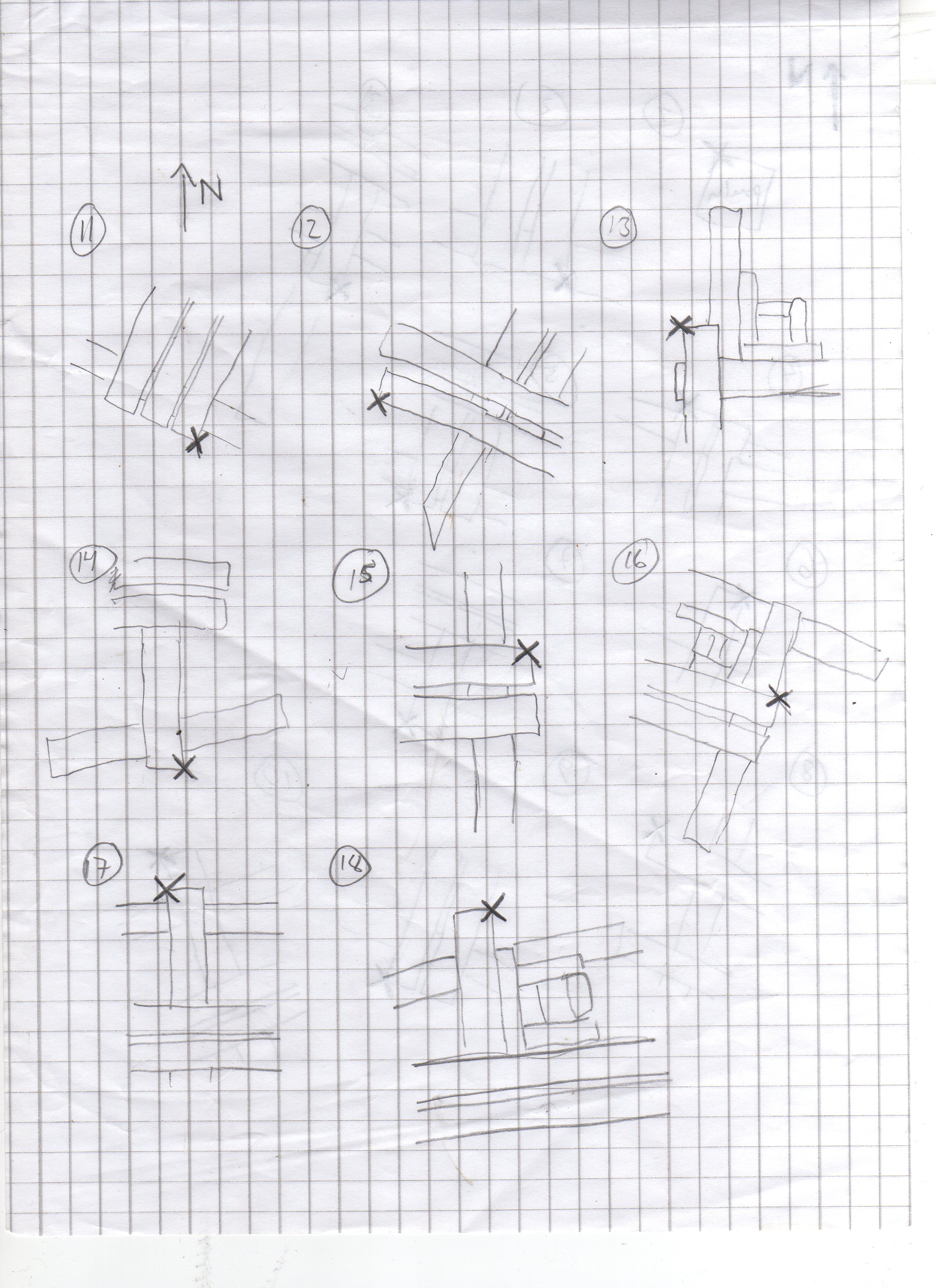
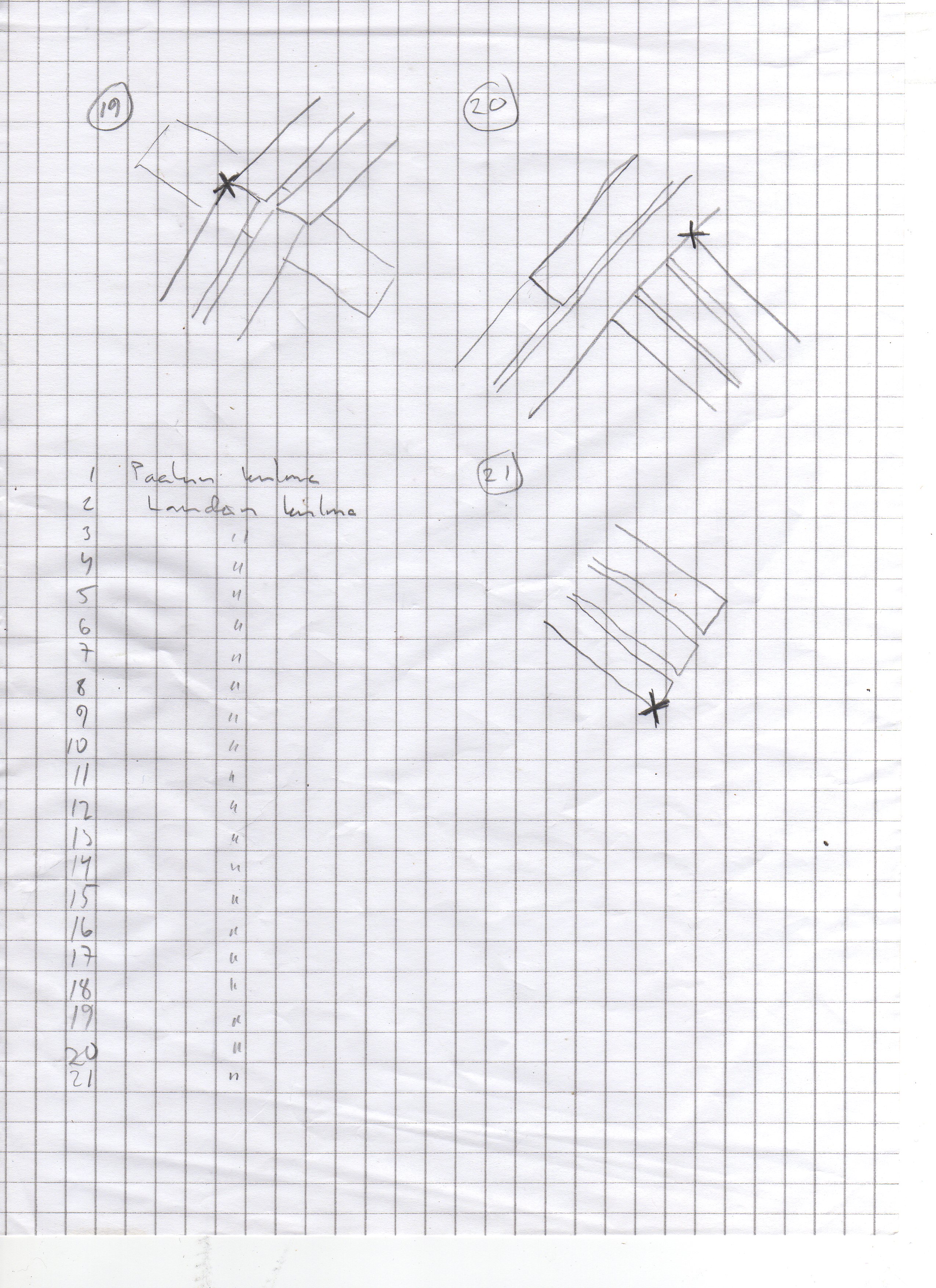
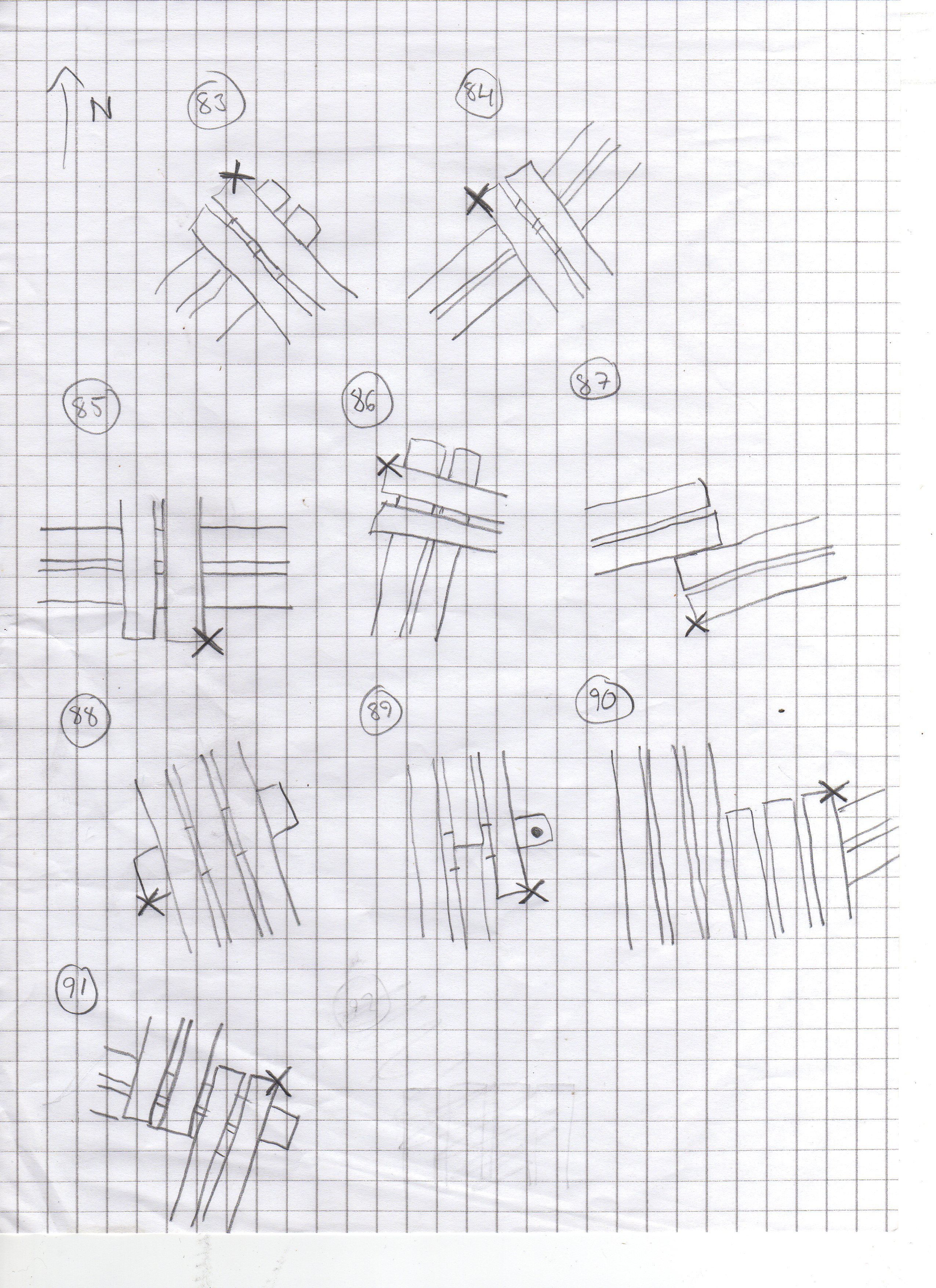
Coordinates of the sample points measured with GNSS (csv).
4.2 Optical propertiesSelected fresh-looking, green canopies. The leaves were already yellowish in most parts of the stand due to the dry season.
Shoots (1-3) from each location were cut and brought to the laboratory. For raspberry, separate samples of 1st year and 2nd year shoots were selected.
While waiting for the measurements, the shoots were kept in a cooling room (7 ºC), in a bucket of water, the lights on.
The maximum time between cutting the shoots and making the measurement was ~4 hours.
Coordinates of the sample points measured with GNSS (csv).
 Raspberry 1 Height 1.55 m, canopy cover (visual esimate) 80% Next to the road, slope towards NW, open area. |
 Raspberry 2 Height 1.20 m, canopy cover 85% Fertile site, alongside a ditch, open area. |
 Raspberry 3 Height 1.1 m, canopy cover 75% Next to a mature forest stand, trees partly shading from the S side. |
 Raspberry 4 Height 1.3 m, canopy cover 75% Next to a mature forest, trees on the S side, 7 m from the sample point. |
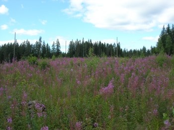
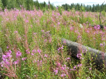
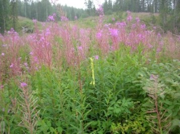 Fireweed 1 Height ~1.5 m, canopy cover 80% Open area, dense canopy. |
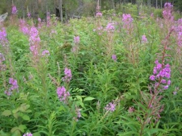 Fireweed 2 Height ~1.5 m, canopy cover 80% Open area, dense canopy. |
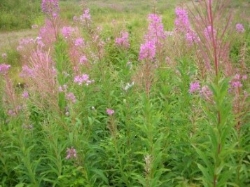 Fireweed 1 Height ~1.5 m, canopy cover 70% Open area, less dense. |
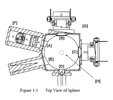
Measured directional-hemispherical
reflectance and transmittance factors (DHRF/DHTF) at 350-2500 nm, using
ASD FieldSpec 3 PRO spectroradiometer and ASD RTS-3ZC integrating
sphere.
Notation for naming the samples:
- sample location
- year class (1 = 1st year, 2 = second year; for raspberry only)
- canopy position (E = sun exposed, S = shaded)
Example:
Raspberry: 1.2.E = location 1, 2nd year shoot, sun exposed
Fireweed: 1.S = location 1, shaded
One fresh-looking leaf representing each sample was selected, detached from the shoot and measured right after the detachment.
4 measurements per sample were taken (reflectance and transmittance, both sides of the leaf).
Work order in the measurements was following:
- putting on the spectrometer, heating the lamp (~30 min before the measurements)
- optimization of the spectrometer i.e. the integration time is adjusted so that the whole DN range (16-bit) is used<>
- measuring the samples:
- for each measurement, 30 readings were taken and averaged
- each measurement stored in a separate file, see the measurement log for file names
- transmittance measurement was repeated 5 times for each sample, by detaching and attaching the leaf to the sample port at each time (this was done because variation was observed between transmittance measurements)<>
- calculation of the reflectance/transmittance factors: DHRF/DHTF = (measured DN - nearest stray light) / (nearest white reference - nearest stray light)
- stray light was measured at the beginning and at the end of measurements
- white reference (separately for each measurement mode) was measured for every other sample
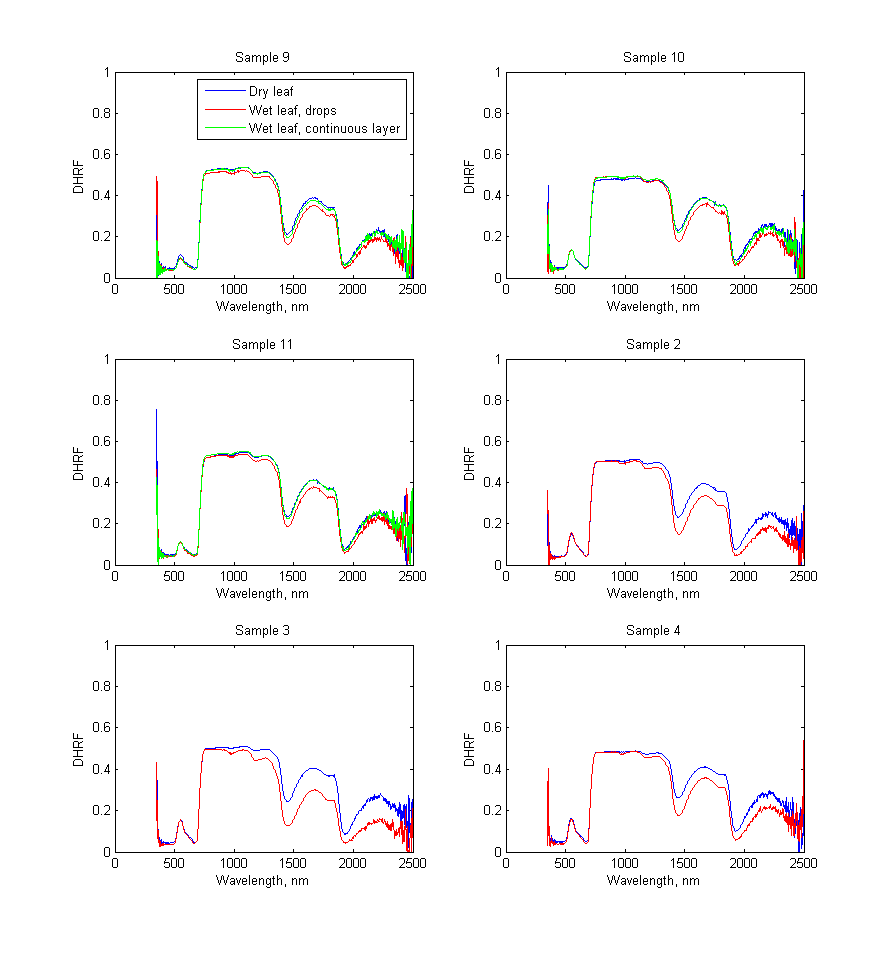
In addition to the basic samples, effect of moisture on raspberry leaf reflectance was tested by spraying the leaf with water.
Measurement log (xlsx).
Port configuration of the integrating sphere and the measurement modes (xlsx) (illustration).
Matlab code for processing the samples (file).
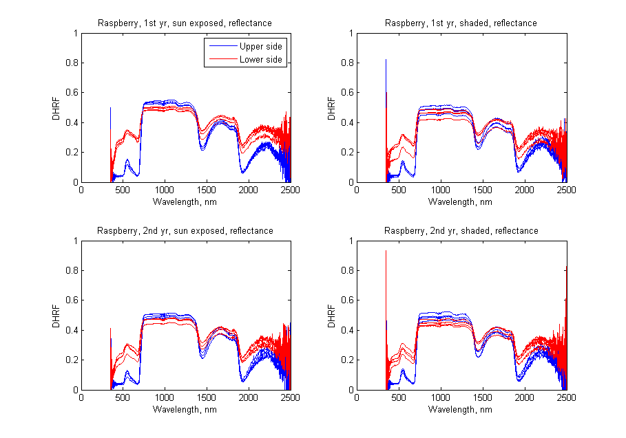
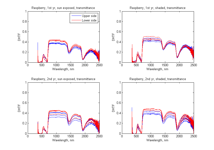
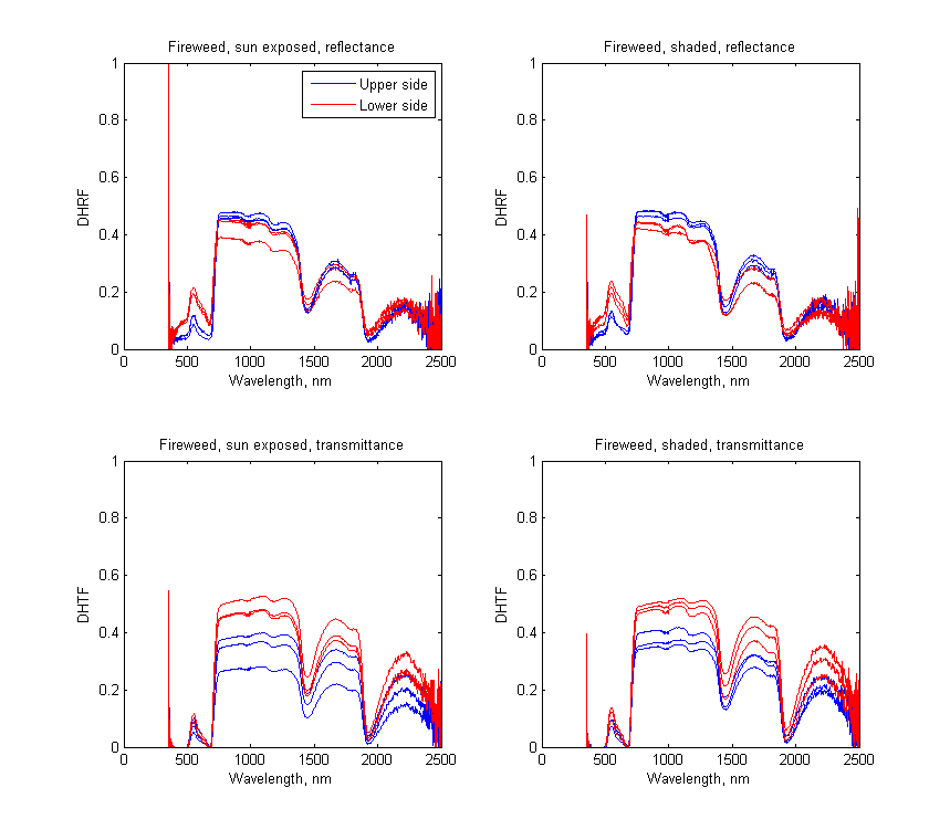
Reflectance spectra of raspberry (fig), transmittance spectra of raspberry (fig), reflectance and transmittance spectra of fireweed (fig).
Effect of moisture on raspberry leaf reflectance (fig)
Measurement data (ASD raw files and exported ASCII). ASD raw files can be readed with ViewSpecPro software (download).
Calculated spectra for the samples (xlsx), calculated after the measurements, no smoothing or cleaning of the outliers. Especially in the transmittance data should be studied more carefully.
Notation for naming the samples:
- sample location
- year class (1 = 1st year, 2 = second year; for raspberry only)
- canopy position (E = sun exposed, S = shaded)
Example:
Raspberry: 1.2.E = location 1, 2nd year shoot, sun exposed
Fireweed: 1.S = location 1, shaded
One fresh-looking leaf representing each sample was selected, detached from the shoot and measured right after the detachment.
4 measurements per sample were taken (reflectance and transmittance, both sides of the leaf).
Work order in the measurements was following:
- putting on the spectrometer, heating the lamp (~30 min before the measurements)
- optimization of the spectrometer i.e. the integration time is adjusted so that the whole DN range (16-bit) is used<>
- measuring the samples:
- for each measurement, 30 readings were taken and averaged
- each measurement stored in a separate file, see the measurement log for file names
- transmittance measurement was repeated 5 times for each sample, by detaching and attaching the leaf to the sample port at each time (this was done because variation was observed between transmittance measurements)<>
- calculation of the reflectance/transmittance factors: DHRF/DHTF = (measured DN - nearest stray light) / (nearest white reference - nearest stray light)
- stray light was measured at the beginning and at the end of measurements
- white reference (separately for each measurement mode) was measured for every other sample
In addition to the basic samples, effect of moisture on raspberry leaf reflectance was tested by spraying the leaf with water.
Measurement log (xlsx).
Port configuration of the integrating sphere and the measurement modes (xlsx) (illustration).
Matlab code for processing the samples (file).
Reflectance spectra of raspberry (fig), transmittance spectra of raspberry (fig), reflectance and transmittance spectra of fireweed (fig).
Effect of moisture on raspberry leaf reflectance (fig)
Measurement data (ASD raw files and exported ASCII). ASD raw files can be readed with ViewSpecPro software (download).
Calculated spectra for the samples (xlsx), calculated after the measurements, no smoothing or cleaning of the outliers. Especially in the transmittance data should be studied more carefully.
4.3 Specific leaf area
Specific leaf area was measured for the
same sample shoots as for optical properties measurements. Same
notation in sample naming used.
Weighing of the leaves,
scanning, drying in 80 °C oven for at least 24 hours.
Scanned images thresholded at blue channel using Otsu's method, and the projected leaf area was determined from the thresholded image.
Specific leaf areas for the samples (xlsx).
Scanned images thresholded at blue channel using Otsu's method, and the projected leaf area was determined from the thresholded image.
Specific leaf areas for the samples (xlsx).