On each 11.28-m circular plot, all photo-trees and trees with dbh > 50 mm are tallied. Sub-sets of trees are sampled to be observed for height, crown length and crown width.
- Plot center. A GPS that gives a ± 1-m accuracy has
been used for determining the plot centers in the field (work done in advance,
we have a limited number of accurate GPS-receivers). The investigators have
a low-quality GPS for finding the plot within ± 10-m accuracy.
The exact plot center is found using triangulation and trilateration. It
needs to be determined with an accuracy of about ± 0.3 m in XY. Each
tree label has the distance and azimuth
from the center. With 2-3 photo-trees the 0.3 m accuracy should be achieved.
- GPS-offset [azimuths and distances]
When the plot and its trees are found, it is possible to measure the vector from the GPS-position to the plot center. We do it by taking interpoint distance and azimuth observations from the photo-trees to the GPS-location that is marked in the field.
- Tree ID [#]
Each tree must have a unique ID that consists of plot ID and a tree ID, which are both numbers.
The numbering of the photo-measured trees follows the azimuth order. The numbering has gaps and does not necessarily start from n:o 1, because all trees, also those surrounding the plot were numbered and printed on the tree map (Fig. 1).
Omission errors, i.e. non-seen trees need to be given an ID in the field. Their numbering should start from e.g. "201" to avoid confusion by duplicates.
Ghost trees: if a photo-tree is found to be in a completety wrong position - off by more than 1 meter and/or the photo-height is wrong by several meters, this tree is rejected and given a new ID.
- Positioning, KKJ [m] (X,Y)
Photo-trees that seem to be in the correct position are letf as is.
All complementary trees are positioned with respect to the photo-trees using the intertree azimuth and distance observations.
These are the unseen and the ghost trees.
The default direction of observation is always from the unknown towards the photo-tree. The photo-tree ID and the distance and/or azimuth are recorded. If the compass-correction (difference between KKJ north and compass north) varies a lot between compasses and investigators, this should also be noted.
We position standing stems at the 1.3-m height, which defines inclusion to the circular plot. For slanted photo-trees the treetop position is decisive.
- Species [class], Sp
The following codes are used. The list may not be complete. If there are exotic species (larches, firs, spruces, pines etc.) encountered, the free codes are taken into use and used consistently by the field group.
1 = pine, 2 = spruce, 3 = pubescent birch, 4 = downy birch, 5 = aspen, 6 = grey alder, 7 = black alder, 8 = Bird cherry, 13 = goat willow, 16 = rowan, 20-25 free codes
- Status [class + written notes]
The status code consists of two digits "##"
11 Living, normal crown
12 Living, crown significantly non-symmetric (e.g. one-sided)
13 Living, crown is damaged / very sparse (dying trees)
14 Living, significantly slanted trunk (> 1 m)
21 Dead tree (recently), standing
22 Dead tree, standing, trunk is broken
23 Dead tree, on the ground (only if a photo-tree has felled between the photography and field work), otherwise we are not interested in fallen trees.
If the tree is exceptional, it is always possible to complete the observation with notes.
- dbh, [mm]
Measured for all trees 1.3 m above ground in [mm]. The measurement direction is perpendicular to a vector that points towards the plot center. I.e. the investigator, when using a caliper, looks towards the plot center.
- height, [m], h
Measured for sample trees that are selected following the every N'th rule. The observation (elevation) angle towards the treetop should be ca. 45 degrees for optimal accuracy (Fig 2).
- height of the lowest living branch, [m], hc
Measured for sample trees that are selected following the every N'th rule. In cases where the lower limit of the crown is uncertain, follow your intuition.
- Maximal crown width, [m] Dcrm.
Measured for sample trees that are selected following the every M'th rule using the Cajanus tube. With it, the investigator observes the plumb line for the crown edge, which is marked on the ground with a metal stick. Two observations from both sides of the stem are made and the distance of the sticks is the estimate for Dcrm.
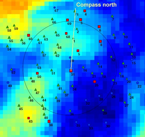
Fig. 2. In taking heigt measurements the device
trembles in the investigators hand (unless we use a tripod or eq.). This roll
of the device causes imprecision that is minimized if the distance to the
tree is equal to the height of the tree minus the observer's height (flat
terrain, 45°).