|
Airborne
data sets on MARV4/2 --- LIDAR
LiDAR 2004 - SPARSE
 The 2004 LiDAR flight was carried out from an airplane travelling
at the speed of 75 m/s. The scanner produced a zig-zag pattern
of pulses. The scanning angle was ± 20º - from an elevation
of 900 m, each 6-km long strip covered a 600-m wide path. Two shorter perpendicular
strips were flown - this was needed for establishing the orientation of the
data - to remove possible systematic offsets in the orientation of the longer
parallel strips.
The 2004 LiDAR flight was carried out from an airplane travelling
at the speed of 75 m/s. The scanner produced a zig-zag pattern
of pulses. The scanning angle was ± 20º - from an elevation
of 900 m, each 6-km long strip covered a 600-m wide path. Two shorter perpendicular
strips were flown - this was needed for establishing the orientation of the
data - to remove possible systematic offsets in the orientation of the longer
parallel strips.The figure below gives a sample of the 2004 LiDAR points superimposed in an image pair. The HSV-coloring is scaled from 0 to 20 meters above ground i.e. the terrain elevation has been checked for each point from the DTM before the HSV-color has been determined. The images are 17 x 17 m and the area is under two parallel strips. 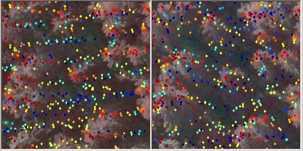
|
LiDAR 2006 - SEMI-DENSE
 The 2006 data set was collected from an airplane travelling at 75 m/s. In
order to get a semi-dense pattern of 6-9 points per m2, the strips have
55% overlap. The instrument could record up to 4 echoes from a pulse. The
data is in so-called comprehensive format, which means that for each pulse
we know the LiDAR-position, attitude in Euler angles, time,
scan angle, and the positions and intensities of the four echoes. This yields
207 bytes per pulse. There can be upto 20 MBytes of data per hectare. The
data is stored in binary files, one file for each KKJ-hectare.
The 2006 data set was collected from an airplane travelling at 75 m/s. In
order to get a semi-dense pattern of 6-9 points per m2, the strips have
55% overlap. The instrument could record up to 4 echoes from a pulse. The
data is in so-called comprehensive format, which means that for each pulse
we know the LiDAR-position, attitude in Euler angles, time,
scan angle, and the positions and intensities of the four echoes. This yields
207 bytes per pulse. There can be upto 20 MBytes of data per hectare. The
data is stored in binary files, one file for each KKJ-hectare. Sample of the semi-dense 2006 data is given below. 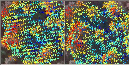
|