Laserkeilauksella tuotetun maastomallin tarkkuus puustoltaan ja topografialtaan erilaisissa kohteissa
Evaluation of the accuracy a lidar-DTM produced fully automatically in targets with varying vegetation and topography
4) Tutkitaan lidar DTM:n tarkkuutta taimikoissa tekemällä referenssimittaukset "taannehtivasti ja metsänhoitajalle sopivalla arvolla" wanhoilta ilmakuvilta. Study the accuracy of the (un-edited) Terramodeler DTM in young stands "retrospectively in a manner fit for the status of a forester" using old aerail photographs.
Puoli-automaattinen apuväline maapisteiden mittaamiseen |
Semi-automatic tool for the measurements of ground points
1. Yhden pisteen mittaus. Simple tool for semi-automatic measurements of single ground points selected by the operator
Maapisteiden osoittaimen useammalta kuvalta on työlästä. Voit käyttää ao. kahta aliohjelmaa mittausten nopeuttamiseksi. Lisää Menu-editorilla valikkokomento Name: "Get_Surface_Height" nimeltään Caption: "Get surface height by image correlation" ja anna sille shortcut painikkeeksi "Del". Manual measurements are laborious. You can insert the two subroutines to KUVAMITT and speed up manual photogrammetric measurements of ground points.
Lisää ao. koodi syntyneeseen vakikko-aliohjelmaan Get_Surface_Height_Click(). Lisää ristikorrelaation laskeva aliohjelma c_cor() MODULE1.BAS ohjelmaikkunaan.
Nyt voit tehdä puoliautomaattisia mittauksia kuvaparilta sirten, että osoitat vain vasemmalta kuvalta pistettä ja painat "Del" näppäintä. Ohjelma tutkii kuvakorrelaation avulla millä korkeudella, vasemman kuvan kuvasäteen 3D kulku-uralla, oikealla kuvalla on "samanlainen maisema". Voit muuttaa kuvaikkunan kokoa (nyt 21 x 21 pikseliä), hakuavaruuden syvyyttä (nyt ± 7.5 m 3D ratkaisun Z:n ympärillä) ja voit muuttaa testipisteiden tiheyttä (nyt pysähdytään 0.1 m välein Z-suunnassa, lasketaan XY(Z) ja kuvakorrelaatio). With these "add-ins'" you can perform semi-automatic measurements by just pointing ground points in the left image and pressing the shortcut key. The program now uses image correlation in determining the XYZ point in the object space where the view in the right image matches that of the left image. The size of the template image windows is 21 by 21 by default, the image-ray of the left image is discretized into XYZ points ±7.5 m in Z (with respect to the Z of the current 3D solution), and the discretization takes place at every 0.1 m in Z. The defaults can be changed.
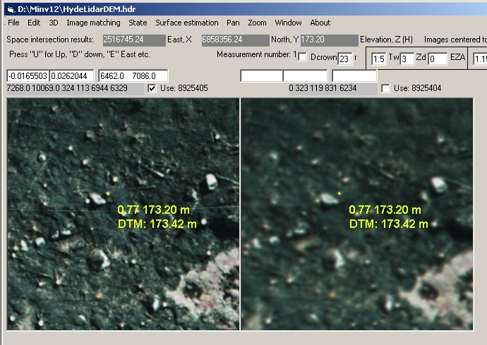
Kuva: Kantoa on osoitettu
vasemmalla kuvalla ja maksikorrelaatio 0.77 on saavutettu korkeudella
173.20 m, jossa vasemman kuvan kuvasäteen X ja Y saavat arvot (2516745.24,
6858356.24) 3D ratkaisu tulostuu keltaisena pisteenä kuville. DTM antaa
ko.pisteessä arvon 173.42 m. Laskenta vie 0.5 sekuntia. Ratkaisun voi
tallentaa normaalisti Shift-F12 -toiminnolla. Huomaa, ettei kuvaa 1 ole klikattu
(tekstiruuduissa ei ole kuvakoordinaatteja). Huomaa, ettei
menetelmä anna yhtä hyviä tuloksia kuin käsin mittaus,
sillä mittausta ei tehdä osapikselitarkkuudella, kuten on mahdollista
käsin mitattaessa zoomia käytettäessä.
An example, where in the left view a stump was
pointed (clear cut photographed three weeks after prescribed burning in
1989), and the maximal correlation, 0.77 is obtained for an XYZ point 173.20
m a.s.l (yellow dots). A lidar based DTM (lidar in 2004) gives an elevation
of 173.42 m in that XY-location. In principle the automatic method will
not yield as accurate results as manual measurements, because sub-pixel-level
computations are not done (cf. zooming the images).
Kuva: Menetemän periaate. Vasemmalta
kuvalta osoitetaan pistettä maassa (punainen piste kuvalla ja maassa).
Kaapataan kuvalta pala maisemaa. Sitten kuvasäde diskretoidaan XYZ-pisteiksi
(mustat), joiden ympäriltä otetaan kuvapaloja oikean puoleiselta
kuvalta. Vasenta kuvapalaa verrataan kaikkiin oikeanpuoleisiin ja saadaan
korrelaatiofunktio, jonka globaalin huipun uskotaan olevan ratkaisussa. Principle of the method.
Kuva: Pari tallennettua korrelaatiofunktiota
(mittausta). Jos Z:aa haluaa tarkentaa, voi huipun ympäristöä
interpoloida ja painottaa esim. kahta ratkaisua (XYZ-pistettä) optimin
(maksimin) ympäriltä. Two examples of correlation
functions (measurements). It is possible to interpolate around the maximal
value and thereby improve the results ('sub-pixel' operation). The horizontal
axis is the Z axis, but recall that for each point the XY-coordinates are
determined by the camera ray of the left view.
Kuva: Tein EH1:n
kuvio 4 maapistemittaukset 1989 kuvilta
uudelleen tällä algoritmilla s.e. vain osoittelin maapisteitä
melkoisella vauhdilla ja tallensin pisteen, jos korrelaatio oli yli 0.75.
248 pisteeseen meni viitisen minuuttia. Residuaalit suhteessa LidarDTM:n
olivat verrannolliset käsinmittauksiin (188 pistettä), itse asiassa
harha oli sama 20 cm, mutta hajonta aavistuksen pienempää! I tried again measuring the required 200 reference ground
points with the algorithm at hand. The results were promising. measuring
248 points took 5 only minutes and the accuracy was comparable to the previously
measured 188 points in which the corresponding ground points were positioned
manually. The bias of the DTM was 20 cm for both points sets and actually
the semi-automatically measured points had a slightly lower stdev.
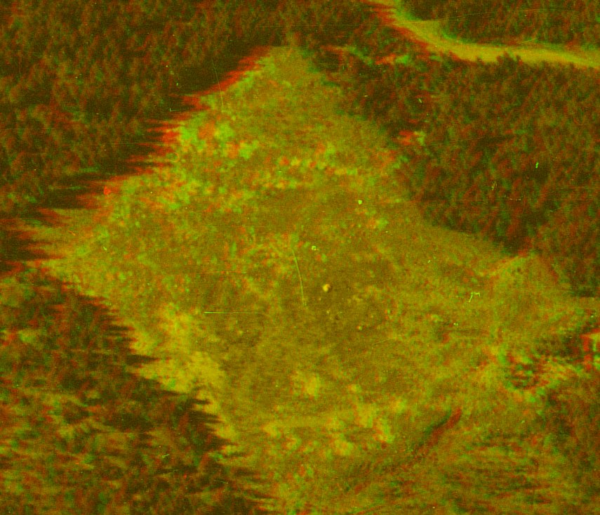
Kuva: Anaglyfikuva aukosta, jossa lokaali DTM tehtiin laskemalla korrelaatiotekniikalla automaattisesti. 3D view from 1973 into the clear cut area subject to retrospective DTM generation.
Kuva: TIN korkeuden mukaan sävytettynä. Orientaatio +- sama kuin anaglyfikuvassa. Kuva tehty Trinet ohjelmalla © Pixel topography Group. The TIN with facets colored by elevation (and shaded). The orientation is made comparable with the anaglyph view above.
2A Lisäpisteitä osoitetun pisteen
ympäristöstä. Searching for (any) points
in the neighborhood
Kuva: Kuvasäteen voi antaa "vaellella osoitetun
pisteen" ympäristössä ja mitata samalla useampia pisteitä.
Tässä osoitetun pisteen (vasemman kuvan) kuvakoordinaatteja on
liikuteltu 200 mikronin hilassa kuvilla on vuodelta 1973 (mittakaavassa 1:22000
15/23 cm kamera). 200 mikronia vastaa noin 4.4 m. Then
I tried the following: allow the image-ray of the left image "float around"
i.e. take values around the pointed target in the image, systematically,
here in a 200 µm image-grid which corresponds to 4.4 m XY-movement
in the object space. I tested with a color image pair from 1973 in scale
1:22000.

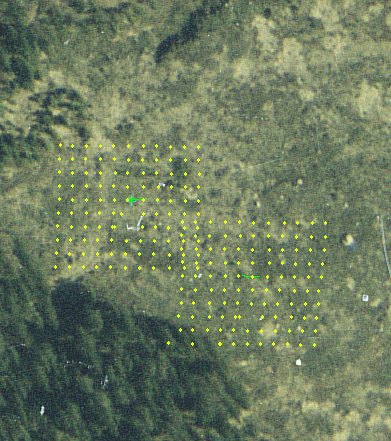
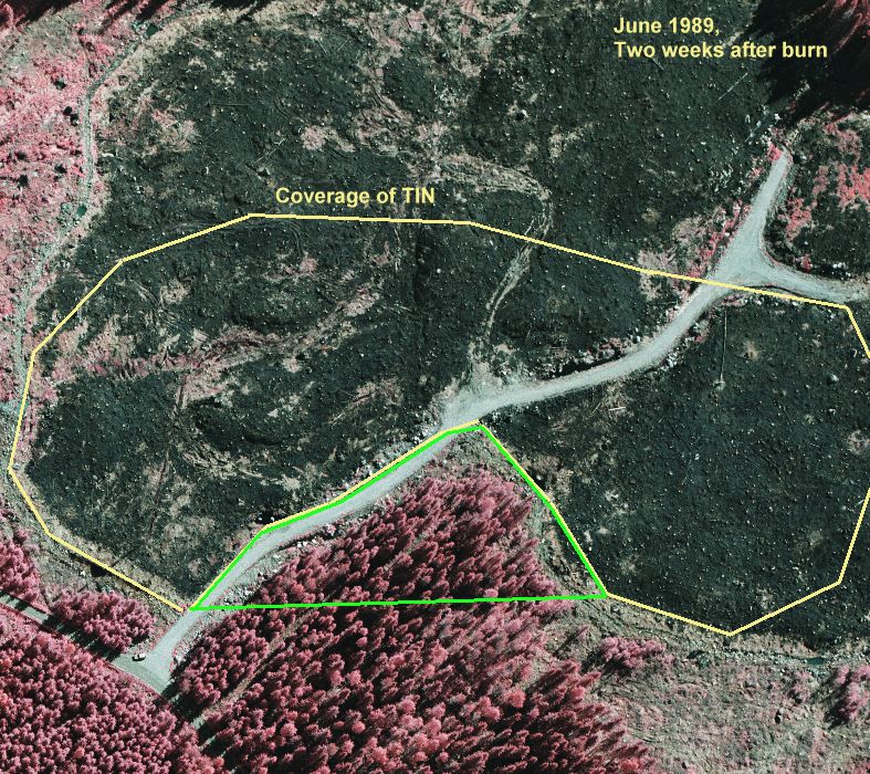
Kuva: noin 200 x 150 metrinen tuore aukko (vrt. anaglyfikuva alla), ja sieltä kuvakorrelaatiolla (> 0.75) löydetyt pisteet sekä niistä laskettu TIN-malli. Tekstuuri alueen keskellä on heikkoa, eikä sieltä saatu montaa korrelaatioltaan > 0.75 pistettä ja TIN jäi harvaksi yrityksistä huolimatta. Kuva tehty Trinet ohjelmalla © Pixel topography Group. By measuring manually about 15 seed positions and then letting the algorithm locate the ground around them, some 300 ground points were quickly measured in a clear cut area of 200 by 150 m. The points with correlation above 0.75 were only accepted and this resulted in an uneven distribution of points that reflects the texture in the images. (cf. anaglyph image below)
Kuva: noin 200 x 150 metrinen tuore aukko (vrt. anaglyfikuva alla), ja sieltä kuvakorrelaatiolla (> 0.75) löydetyt pisteet sekä niistä laskettu TIN-malli. Tekstuuri alueen keskellä on heikkoa, eikä sieltä saatu montaa korrelaatioltaan > 0.75 pistettä ja TIN jäi harvaksi yrityksistä huolimatta. Kuva tehty Trinet ohjelmalla © Pixel topography Group. By measuring manually about 15 seed positions and then letting the algorithm locate the ground around them, some 300 ground points were quickly measured in a clear cut area of 200 by 150 m. The points with correlation above 0.75 were only accepted and this resulted in an uneven distribution of points that reflects the texture in the images. (cf. anaglyph image below)
Kuva: Anaglyfikuva aukosta, jossa lokaali DTM tehtiin laskemalla korrelaatiotekniikalla automaattisesti. 3D view from 1973 into the clear cut area subject to retrospective DTM generation.
Kuva: TIN korkeuden mukaan sävytettynä. Orientaatio +- sama kuin anaglyfikuvassa. Kuva tehty Trinet ohjelmalla © Pixel topography Group. The TIN with facets colored by elevation (and shaded). The orientation is made comparable with the anaglyph view above.
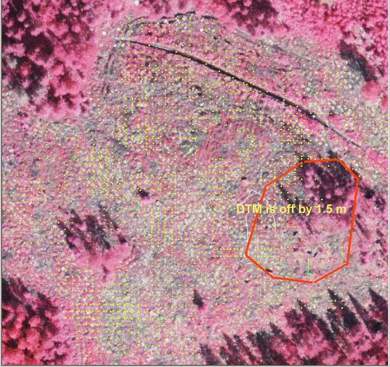
Kuva: Vuoden 2004 kuvaparilta (1:14000 21/23
60%) mitatut maapisteet, r > 0.8. Aukkoja jää puustoisiin
kohteisiin ja tekstuuriltaan tasaisiin alueisiin. Another
example with images from 2004, two weeks prior to the lidar campaign. 1726
points with correlation above 0.8 ssuperimposed in the image. Note again
the sparse areas where texture is low.
Kuva: Jokaiselle kuvaparilta autom. mitatulle
pisteelle (N=1726) on laskettu ero LidarDTM:n suhteen. The automatically measured gournd points were checked for
Z using the TeraModeler DTM, here are the differences. There is a large
40 x 40 m area, where the differences are large.
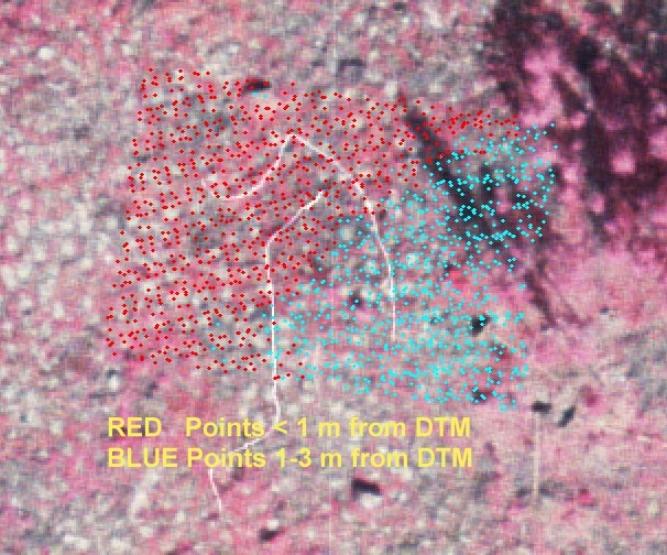
Kuva: Ilmakuvalle, kohtaan, jossa erot ovat
suuria, on tulostettu pisteet, jotka ovat alle 1 m LidarDTM antamasta korkeudesta
ja toisaalta pisteet, jotka ovat 1-3 m pinnasta. Jostain syystä TerraModeler
on tuottanut isohkon virheen DTM:ään (vaikka kyseessä on
aukea/1-v taimikko), joka näin paljastui autom. kuvamittausten avulla.
When the individual raw lidar observations were
superimosed in the images it could be sen that the DTM is erroneous in that
part where the differences were large.
2B Rajautuminen tekstuuriltaan mielenkiintoisiin kuvan kohtiin Searching for interesting points in the neighborhood
Mikäli kuvakorrelaatiota lasketaan mille tahansa kuvapisteelle, muodostavat tasaisen tekstuurin alueet ongelmia. Ao. kuva olkoon esemerkkinä. Image-matching fails in areas of low contrast.
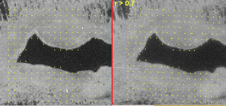
Kuva: Jos kuvakorelaatio lasketaan tekstuurittomasta
kuvasta (pinnasta), saadaan hyvin huonoja tuloksia (kts. alla). Kuvassa nevan
ympäröimä (aivan tasainen) metsälampi. Löydetyt 3D
pisteet eivät muodosta tasavälistä hilaa oikealla kuvalla kuten
pitäisi olla maaston tasaisuuden perusteella. If
the corralation is computed for surfaces with low texture, the results are
bad (see below). Here, an open, treeless bog surrouns a small pond.
The surface is flat, but the matched points do not form a regular grid in
the right image.
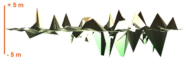
Kuva: Näkymä "suoraan horisontista
/ sivulta" 1962 kuvamittauksien (kuva yllä) perusteella tehtyyn DTM-malliin.
Tasaisen tekstuurin alueella on pahoja virheitä. The resulting erroneus TIN-DTM as seen from "the side".
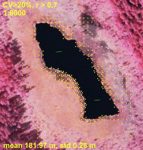
Kuva: Kun sama alue mitataan 1:8000 väri-infrakuvilta
saadaan enemmän pisteitä, ilmeisesti kuvien paremman tekstuurin
takia. Silti nevalle (rahkanevaa - lyhytkorsinevaa - ei kuljuja) jää
suuria aukkoja, joista ei saada havaintoja. Here, the
same area was measured in an image pair in the scale of 1:8000. These images
have better texture.
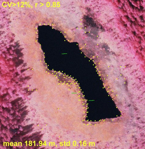
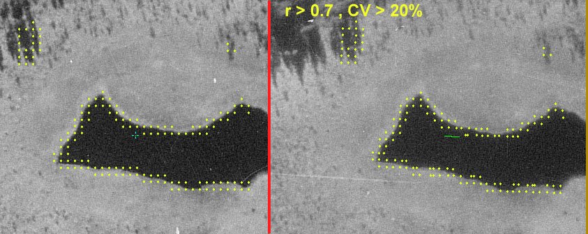
Kuva: Tässä vaadittua korrelaatiota on kiristetty tasolle 0.85,
ja vaikka CV-rajoite (tekstuuri) on laskettu 12% saadaan vähemmän,
mutta tarkempia pisteitä.
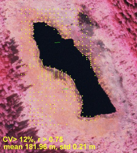
Kuva: Korrelaatio on laskettu tasolle 0.75, mikä
aiheuttaa pisteiden lisääntymisen. Tarkkuus on edelleen kohtuullinen,
hajonta 21 cm yli keskiarvon (suon voi olettaa olevan tasainen).
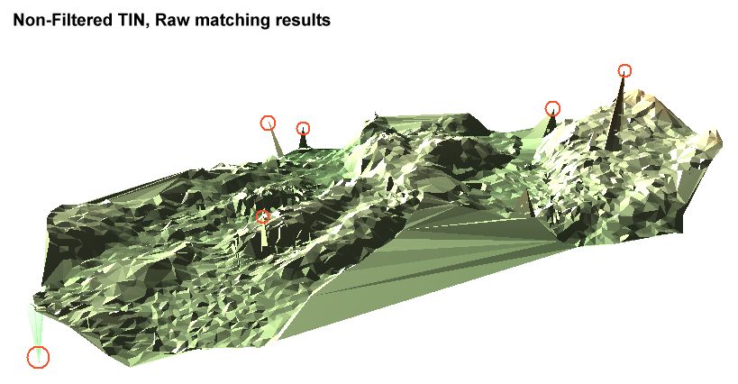
Kuva: 4900 pisteeseen laskettu TIN-malli, jossa näkyy kuvien yhteensovituksessa tapahtuneita virheitä - teräviä piikkejä ylös ja alas. With correlation coefficient limited at 0.75 the data still contained erronous solutions, which show in the TIN-DTM as peaks (up and down).
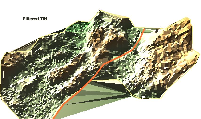
Kuva: Piikkipisteet on suodatettu tutkimalla jokaisen pisteen osalta kaikki kolmiot, joissa piste on solmuna. Jos kaikkien kolmioiden pinnan normaalivektorit osoittivat "kohti horisonttia tai sinne päin", kyseessä on piikin aiheuttanut piste, eli virhehavainto, joka yksinkertaisesti jätettiin pois kuvan TIN laskettaessa. Maaston korkeus vaihtelee välillä [167.4, 177.4 m]. A simple filtering of the peaks was carried out by checking for each noode-point the orientation of the triangle facets. If all facets "faced the horizon" that point was simply rejected. Here the resulting DTM has a range from 167.4 to 177.4 m a.s.l.
Private Sub Get_Surface_Height_Click()
Rem Point a target in image(0)
Rem Routine computes the path of the ray, solves for XYZ, when Z takes values around
rem the current solution of Z
Rem Routine captures a template in image 0 around the image position pointed
Rem For all XYZ points along the camera ray of the image(0), the template is checked for
Rem correlation with image(1). Maximum correlation r [-1,1] occurs at certain XYZ position,
Rem which is made the 3D solution
Dim Index As Integer, Z_gnd As Double, X_gnd As Double, Y_gnd As Double
Dim p_x As Double, p_y As Double
Dim R_tau(1 To 200, 4) As Double, Rmaxind As Long
Rem Always use the image(0) upper-left, i.e. set index to zero
Index = 0
Rem If there is no solution, start looking around 160 m a.s.l.
If SolutionExists = False Then Z_sol = 160
Rem Assign the test variable Z_gnd with initial value, center of the search in Z
Z_gnd = Z_sol
Rem Solve XY for the given Z and image observation of left image
Call solve_3D_X_Y_from_Z_x_y(Index, Z_gnd, CDbl(Text1(Index * 2).Text), CDbl(Text1(Index * 2 + 1).Text), X_gnd, Y_gnd)
Rem SOlve position in the pixel coordinates
Call r_transform_ground_to_pixel(Index, X_gnd, Y_gnd, Z_gnd, p_x, p_y)
Rem Get pixels of the reference template. bkuva() -RGBtriplet array
Rem Vary template size (square) is necessary
TempWidth = 21
Rem *** SECTION FOR FILLING THE TEMPLATE bkuva() WITH PIXEL-values, starts here **
ReDim RROW(0 To (TempWidth - 1)) As RGBtriplet
Close (2)
Open image_info(Index).filename For Binary As 2
startrow = (image_info(Index).sub_height - 1) - p_y - TempWidth / 2
startcol = p_x - TempWidth / 2
endcol = startcol + (TempWidth - 1)
ReDim bkuva(0 To (TempWidth - 1), 0 To (TempWidth - 1)) As RGBtriplet
k = -1
For i = startrow To startrow + (TempWidth - 1)
k = k + 1
paikka = CLng(i) * CLng(image_info(Index).sub_width) * 3 + CLng(startcol) * 3
Rem Read a row
Get #2, paikka + 1, RROW()
kx = 0
For m = 0 To (endcol - startcol)
bkuva(m, k).r = RROW(m).r
bkuva(m, k).g = RROW(m).g
bkuva(m, k).B = RROW(m).B
Next m
Next i
Close (2)
Rem *** SECTION FOR FILLING THE TEMPLATE, bkuva() WITH PIXEL-values, stops here here **
Rem Now we should search for a reference templates in image(1) "right" at
Rem XYZ positions along the image ray of image(0) "left"
Dim Z_test As Double, Z_depth As Double, Z_step As Double
Rem We let Z vary +- Z_depth around the initial value
Z_depth = 7.5
Rem It is image(1) that is the target of template matching
Index = 1
Rem Discretize the image ray by solving for a XYZ position at every Z_step distance in Z
Z_step = 0.1
Dim ix As Long, Rmax As Double
Rem ix is a counter for XYZ points, Rmax is set at -5
ix = 0
Rmax = -5
Rem Start to discretize the image ray of image(0)
For Z_test = Z_gnd - Z_depth To Z_gnd + Z_depth Step Z_step
ix = ix + 1
Rem Solve XY for Z, based on image observation made in the "left" image(0)
Call solve_3D_X_Y_from_Z_x_y(0, Z_test, CDbl(Text1(0 * 2).Text), CDbl(Text1(0 * 2 + 1).Text), X_gnd, Y_gnd)
Rem Solve pixel location
Call r_transform_ground_to_pixel(Index, X_gnd, Y_gnd, Z_test, p_x, p_y)
Rem *** GET PIXELS OF IMAGE1 into ckuva() aRGBtriplet array ***
Open image_info(Index).filename For Binary As 2
startrow = (image_info(Index).sub_height - 1) - p_y - TempWidth / 2
startcol = p_x - TempWidth / 2
endcol = startcol + (TempWidth - 1)
ReDim ckuva(0 To (TempWidth - 1), 0 To (TempWidth - 1)) As RGBtriplet
k = -1
For i = startrow To startrow + (TempWidth - 1)
k = k + 1
paikka = CLng(i) * CLng(image_info(Index).sub_width) * 3 + CLng(startcol) * 3
Rem Read a row
Get #2, paikka + 1, RROW()
For m = 0 To (endcol - startcol)
ckuva(m, k).r = RROW(m).r
ckuva(m, k).g = RROW(m).g
ckuva(m, k).B = RROW(m).B
Next m
Next i
Close (2)
Rem *** GET PIXELS OF IMAGE1 into ckuva() a RGBtriplet array, done ***
Rem r is the correlation coefficient, computed for tempates bkuva() (fixed)
rem and ckuva()which is centered at XYZ positions in image(1)
Dim r As Double
Call c_cor(bkuva(), ckuva(), r)
Rem Check if this is the maximal correlation so far
If r > Rmax Then
Rmaxind = ix
Rmax = r
End If
R_tau(ix, 1) = r
R_tau(ix, 2) = X_gnd
R_tau(ix, 3) = Y_gnd
R_tau(ix, 4) = Z_test
Next Z_test
Rem After checking all positions, assign 3D solution with point that had largest correlation
X_sol = R_tau(Rmaxind, 2)
Y_sol = R_tau(Rmaxind, 3)
Z_sol = R_tau(Rmaxind, 4)
Rem Update Main-form
Form1.Label4(0).Caption = Format$(X_sol, "#.00")
Form1.Label4(1).Caption = Format$(Y_sol, "#.00")
Form1.Label4(2).Caption = Format$(Z_sol, "#.00")
Rem Update measurement -structure
Measurement.Num = MeasurementCounter
Measurement.X = X_sol: Measurement.Y = Y_sol: Measurement.z = Z_sol
Rem RMSE is now correlation
Measurement.RMSE = R_tau(Rmaxind, 1)
Rem Get DTM-elevation
Measurement.z_DTM = getheight(X_sol, Y_sol)
Rem Rem superimpose the point in the images 0 "left" and 1 "right", print the correlation and
Rem Z for the solution and Z from the DTM
For i = 0 To 1
Call r_transform_ground_to_pixel(i, R_tau(Rmaxind, 2), R_tau(Rmaxind, 3), R_tau(Rmaxind, 4), p_x, p_y)
Form1.Picture1(i).DrawWidth = 3
Form1.Picture1(i).Cls
Form1.Picture1(i).PSet ((p_x - (image_info(i).o_col + win_info(i).win_o_col)) * win_info(i).pan_x - 1, ((image_info(i).Height - 1) - p_y - (image_info(i).o_row + win_info(i).win_o_row)) * win_info(i).pan_y), RGB(225, 255, 25)
Form1.Picture1(i).FontSize = 12
Form1.Picture1(i).ForeColor = RGB(225, 255, 25)
Form1.Picture1(i).CurrentX = Form1.Picture1(i).CurrentX + 15
Form1.Picture1(i).CurrentY = Form1.Picture1(i).CurrentY + 15
Form1.Picture1(i).Print Format$(R_tau(Rmaxind, 1), "0.00") & " " & Format$(R_tau(Rmaxind, 4), "#.00 m")
Form1.Picture1(i).PSet ((p_x - (image_info(i).o_col + win_info(i).win_o_col)) * win_info(i).pan_x - 1, ((image_info(i).Height - 1) - p_y - (image_info(i).o_row + win_info(i).win_o_row)) * win_info(i).pan_y), RGB(225, 255, 25)
Form1.Picture1(i).CurrentX = Form1.Picture1(i).CurrentX + 15
Form1.Picture1(i).CurrentY = Form1.Picture1(i).CurrentY + 35
Form1.Picture1(i).Print "DTM: " & Format$(Measurement.z_DTM, "#.00 m")
Form1.Picture1(i).DrawWidth = 1
Next i
End Sub
Koodi Module1.BAS ohjelmaikkunaan
Public Sub c_cor(ima1() As RGBtriplet, ima2() As RGBtriplet, r As Double)
Dim os As Double, nim1 As Double, nim2 As Double, meanA As Double, meanB As Double
os = 0#
nim1 = 0#
nim2 = 0#
meanA = 0#
meanB = 0#
Dim i As Long, j As Long
If UBound(ima1, 1) <> UBound(ima2, 1) Then
MsgBox ("Templates are of unequal size!")
End If
For i = 0 To UBound(ima1, 1)
For j = 0 To UBound(ima1, 2)
meanA = meanA + ima1(i, j).g
meanB = meanB + ima2(i, j).g
Next j
Next i
meanA = meanA / (UBound(ima1, 1) * UBound(ima1, 2))
meanB = meanB / (UBound(ima2, 1) * UBound(ima2, 2))
For i = 0 To UBound(ima1, 1)
For j = 0 To UBound(ima1, 2)
os = os + (CDbl(ima1(i, j).g) - meanA) * (CDbl(ima2(i, j).g) - meanB)
nim1 = nim1 + (CDbl(ima1(i, j).g) - meanA) * (CDbl(ima1(i, j).g) - meanA)
nim2 = nim2 + (CDbl(ima2(i, j).g) - meanB) * (CDbl(ima2(i, j).g) - meanB)
Next j
Next i
If ((nim1 * nim2) < 0.002) Then
r = -2#
Exit Sub
End If
r = 1 * os / Sqr(nim1 * nim2)
End Sub