Erikoisharjoitus I Special assignment I
Laserkeilauksella tuotetun maastomallin tarkkuus puustoltaan ja topografialtaan erilaisissa kohteissa
Evaluation of the accuracy a lidar-DTM produced fully automatically in targets with varying vegetation and topography

---

1) Tutkitaan, kuinka tarkan maastomallin pystyy tuottamaan täysin automaattisesti luokittamalla TerraModeler -ohjelmalla "kasvukauden aikaisia" laserpisteitä maapisteiksi varttuneissa puustoissa. Mallina käytetään D:\MINV12\ HydeLidarDEM.hdr tiedostoa.
The objective is to assess the accuracy of a DTM produced "almost automatically" with TerraModeler-software (no editing/post-processing has taken place). The lidar data, 0.7 p /m2, 900 m AGL represent a leaf-on case from August 2004. There are 10900 testpoints (tree butts) in stands > 40 yrs old.

Ohjelmalla Raster_DTM_Eval  lasketut koealakohtaiset tulokset ovat  (Private Sub Open_Dem_File_Click() modifioitu s.e. DTM-korkeuksiin on lisätty 0.18 m, joka puuttuu raakalidar-havainnoista: ZfXY(j, i) = CSng(row(j)) + 0.18
Using the DTM_EVAL-program for computations, with 0.18 m added to the lidar data (observed offset at the GPS-reference of the lidar campaign), the following per field plot results were obtained.

Plot   N  Range   STD Mean(dZ) RMS(dZ)  STD(dZ)
FT     135   2.12 0.49 -0.21   0.24   0.128
KM     128   5.93 1.45 -0.08   0.16   0.141
KO1     96   4.17 1.02  0.22   0.28   0.180
KO2    201   5.57 1.35  0.37   0.41   0.167
KO3     83   3.23 0.80  0.31   0.34   0.143
KO4     83   3.45 0.91  0.03   0.21   0.208
KU1    213   5.83 1.46  0.19   0.30   0.224
KU2    280   5.20 1.17  0.47   0.49   0.148
KU3    527   5.19 1.07  0.37   0.40   0.150
KU4    381   8.28 2.06  0.41   0.50   0.286
KU5    438   7.87 1.44  0.42   0.45   0.166
KU6    246   6.12 1.53  0.10   0.16   0.131
L15    794   2.09 0.41 -0.05   0.13   0.126
L88    691   6.04 0.88  0.09   0.19   0.169
LK1     86   0.53 0.12  0.08   0.11   0.072
LK2    110   1.17 0.31  0.21   0.22   0.076
MA1    318   6.27 1.69  0.13   0.22   0.168
MA2    418   5.81 1.18  0.04   0.15   0.148
MA3    345   3.75 0.84  0.73   0.83   0.398
MA4    432   5.31 1.03  0.33   0.42   0.263
MA6    353   4.18 0.66  0.16   0.25   0.190
MAKU   435   4.94 1.23  0.19   0.25   0.163
MK     267   9.91 2.20  0.26   0.34   0.214
MMM1   580  18.02 6.39  0.13   0.33   0.308
MMM2  2267  13.45 2.11  0.26   0.35   0.237
MMM2   509   8.30 1.91  0.31   0.41   0.269
TELE   525   4.40 1.15  0.12   0.21   0.172

Koealoista MMM1 ja KU4 näyttivät sellaisilta (Range, STD), että niissä on korkeusvaihtelua. Samoin MA3 virheet näyttivät suurilta (RMSE 0.83 m). Näillä koealoilla residuaaleja katseltiin tarkemmin.
Based on the tabulated data it seems that plots MMM1 and KU4 have a more varying topography. Also, the errors of plot MA3 are large. Thus these three plots were examined more carefully.

Yleisesti tulokset ovat melko lupaavia; koealojen maaston muototarkkuus (STD(dZ)) on kaikilla koealoilla alle 0.4 m, yleensä alle 0.3 m. VAR(dZ) ja VAR(Z) välinen suhde indikoi, että DTM pystyy ennustamaan melko suuren osan topografian vaihtelusta.
In all, the results are "promising", since the "accuracy of the relief", STD(dZ), is less than 0.3 m in all plots except for plot MA3. The ratio VAR(dZ) / Var(Z) implies also that the DTM is able to model the relief largely.

C:\DATA\Pointresults.txt kerättiin ko. koealoille xls-tiedostot, jossa oli pisteille X, Y, Z, 0, 0, Z-ero ja ne luettiin Matlabiin (xlsread()-funktiolla). Siellä quiver3() -funktiolla tuotettiin ao. kuvat.
The pointwise residuals in c:\data\pointresults.txt were processed for plotwise xls-files, that had records of [X,Y,Z,0,0,dZ] and these xls-files were imported to Matlab using the xlsread()-function. In Matlab, quiver3()-function was applied for rendering the figures below.

Kuva: residuaalikuva paljastaa, kuinka virheet korreloivat spatiaalisesti ha korkeudet ovat aliarvioituneet (positiiviset ylös osoittavat virhevektorit) erityisesti jyrkässä rinteen osassa. Koealan halkaisee metsäautotie, jonka eteläpuolinen ojitettu räme on tasainen, ja DTM toimii siellä kohtuuullisesti. The 3D residual plot reveals the positive spatial correlation of the errors, and how the errors are largest (elevation is underestimated) in the slopes. The area is partioned by a forest road, and the southern part is made up of a drained pine bog where the topograghy is flat.

Kuva: Suurimmat aliarviot, 1,3 - 1,9 m löytyvät "jonossa" 50x50 m koealan luoteisnurkasta; 3D pistekuvaa pyöritellessä katsellessa huomaa, että koealaln leikkaa 1-2 m korkea kalliojyrkänne, ja puut, joille residuaali on suuri ovat tämän jyrkänteen "terassin päällä". DTM-malli ei osaa "nousta" jyrkänteen päälle kunnolla vaan DTM on suodattanut jyrkänteen. The largest underestimation (errors ni the DTM) of elevation, from 1.3 to 1.9 m are located in the NW-corner of the 50 x 50 m plot. The errors are due to the fact that the DTM did not follow a 2-m high, 15-m long steep . The DTM (1 x 1 m resolution, interpolated from a TIN produced by TerraModeler-software) has smoothed the relief.

Kuva: MA3 residuaalien jakauma on kaksihuippuinen. Suuresssa osassa koealaa erot ovat noin +1 m, koealan kaakkoiskulmassa + 0.2 m. On todennäköisintä, että koealan vaaituksessa on on tapahtunut virhe, esim. s.e. takymetrillä mitatessa on unohdettu antaa prismakorkeus, esim. 1 m, kun konetta on siirretty ja tällöin koko pistejoukko on Z:n suhteen väärässä paikassa. The DTM-errors of plot MA3 have a bimodal distribution. The residuals are mostly near +1 m except for an area in the SE-corner, where the residuals are ~ +0.2 m . It is likely that the reference data contains errors: the levelling in this case by tacheometer. It is easy to make 1 m systematic errors with a tacheometer, if the height of the reflecting prism or the apparatus is set wrong.

Koeala MA 3 löytyy melko pian avohakkuun jälkeen kuvattuna vuoden 1962 ilmakuvilla. Niiltä mitattiin joukko hajapisteitä. Plot Ma3 has been photographed soon after it was clear-cut and regenerated some 50 years ago in 1958-1959. These aerial images were used for getting additional reference data of terrain elevation.


Kuva: 1962 kuvilta (koeala noin 5-vuotiasta taimikkoa) mitattujen maapisteiden (23 kpl) residuaalit dZ [-0.67 m, + 1.18 m ]  keskiarvo(dZ) = +0.32 m, STD(dZ) = 0.47 m plotattuna sinisellä. Analyysi näyttäisi tukevan käsitystä siitä, että takymetrimittaukset maastossa ovat epäonnistuneet. In photographs of 1962, when the pine seedlings were maybe 4-5 years old, 23  terrain points were measured. Their differences (plotted in blue) against the DTM had a range from -0.67 to to +1.18 m with a mean of +0.32 m. This analysis gives support to the assumption that the tacheometer measurements for tree butt elevations have failed.


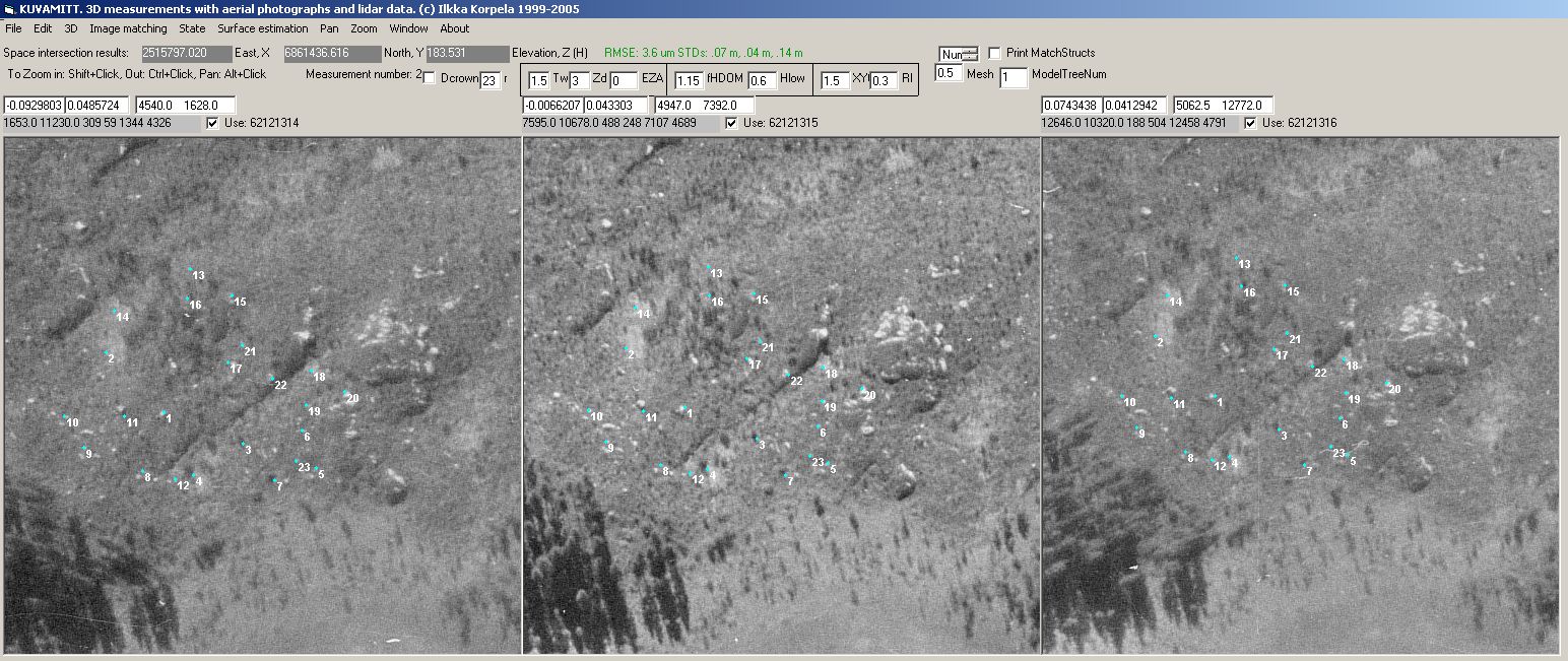
Kuva: referenssipisteet ilmakuvatripletillä vuodelta 1962. The manually measured 23 points seen in an image triplet from 1962.

---

2) Tutkitaan, miten puusto vaikuttaa lidar maaosumien spatiaaliseen jakaumaan. Let's study how trees and other flora affect the spatial pattern of lidar's ground points

Projisoidaan maanpintaa lähellä olevia lidar-pisteitä KUVAMITT-ohjelmalla ilmakuville ja kirjoitetaan ko. pisteitä tiedostoon. Pidetään lidar DTM-mallia oikeana maanpintana. Tutkitaan joitakin (min 3) puustoltaan erilaisia kohteita, oma valinta. Kuvaillaan spat. jakaumia; ilmakuvia tulkitsemalla näkee osin, miksi lidar pulssi ei jatkanut matkaansa maanpinnalle.Superimpose lidar points near to the terrain surface in the aerial images using KUVAMITT-software and at the same time write the data into an ASCII-file. Consider the lidar DTM produced by TerraModeler as the reference. Study a minimum of three locations with varying growing stock, select yourselves. Describe the spatial patterns; using the aerial images you can see, in part, why a particular pulse has not reached  the ground.

Lisäsin erikoisharjoitus 4 Visual Basic ohjelman aliohjelmaan Open_Plot_TreeFile_and_read_lidar_Click() rivit, jotka avaavat ja sulkevat ASCII-tiedoston sekä puiden XYZ koordinaattien että lidar-pisteiden XY ja H (normalisoitu korkeus) koordinaattien tallentamiseksi: I added a few code-lines to the source code of the program for special assignment 4. The subroutine Open_Plot_TreeFile_and_read_lidar_Click() was added commands that open and close ASCII-files for output of XYZ data for trees and lidar points.  
....
Open "c:\data\LK2_trees_KKJ.txt" For Output As 6
Do Until EOF(1)
 i = i + 1
 Input #1, FieldTrees(i).x, FieldTrees(i).y, FieldTrees(i).z, FieldTrees(i).d13, FieldTrees(i).h, FieldTrees(i).Num, FieldTrees(i).Sp, FieldTrees(i).Status
 Rem Depending on how d13 is stored; change code below
  FieldTrees(i).d13 = FieldTrees(i).d13 / 10   ' mm to cm
 Rem FieldTrees(i).d13 = FieldTrees(i).d13 * 100  ' m to cm
 
 xp = Cos(angle) * FieldTrees(i).x - Sin(angle) * FieldTrees(i).y
 yp = Sin(angle) * FieldTrees(i).x + Cos(angle) * FieldTrees(i).y
 Rem Convert local butt coordinates into 3D object coordinate frame
 FieldTrees(i).x = xp + X_origo + X_shift
 FieldTrees(i).y = yp + Y_origo + Y_shift
 FieldTrees(i).z = FieldTrees(i).z + Z_origo + Z_shift
 Print #6, FieldTrees(i).x, FieldTrees(i).y, FieldTrees(i).z
Loop
Close (1)
Close (6)

....puuttuvaa koodia....

Label1.Caption = "Normalizing lidar heights to DTM..."
DoEvents
 Open "c:\data\LK1_normalized_lidar.txt" For Output As 4
 For i = 1 To Mp
 
       LPH(i).GPS_time = LP(i).GPS_time
       LPH(i).Intf = LP(i).Intf
       LPH(i).Ints = LP(i).Ints
       LPH(i).Rangef = LP(i).Rangef
       LPH(i).Rangel = LP(i).Rangel
 '      LPH(i).Xl = LP(i).Xl
 '      LPH(i).Yl = LP(i).Yl
 '      LPH(i).Zl = LP(i).Zl
       LPH(i).Xs = LP(i).Xs
       LPH(i).Ys = LP(i).Ys
       LPH(i).Zs = LP(i).Zs
       LPH(i).Xf = LP(i).Xf
       LPH(i).Yf = LP(i).Yf
       LPH(i).Zf = LP(i).Zf
'       LPH(i).kappa = LP(i).kappa
'       LPH(i).omega = LP(i).omega
'       LPH(i).phi = LP(i).phi
       LPH(i).Scan_angle = LP(i).Scan_angle
  
      Rem Get heights above ground; some first return points have 0-values in raw data
      Rem These have negative Y-values in KKJ
 
      If LP(i).Zs < 0 Then MsgBox ("!")
      
      LPH(i).Hs = 0
      LPH(i).Hf = 0
      
   Rem Check how many actual returns we have; if less than 3 make first = last
      
   LPH(i).Hs = LPH(i).Zs - getheight(LPH(i).Xs, LPH(i).Ys)
  
   Print #4, LPH(i).Xs, LPH(i).Ys, LPH(i).Hs
  
   If Abs(LP(i).Rangef - LP(i).Rangel) < 3 Or Abs(LP(i).Rangef - LP(i).Rangel) > 40 Then
       LPH(i).Xf = LP(i).Xs
       LPH(i).Yf = LP(i).Ys
       LPH(i).Zf = LP(i).Zs
       LPH(i).Hf = LPH(i).Zf - getheight(LPH(i).Xf, LPH(i).Yf)
   End If
      
   If (LP(i).Rangel - LP(i).Rangef) >= 3 And (LP(i).Rangel - LP(i).Rangef) < 40 Then
       LPH(i).Hf = LPH(i).Zf - getheight(LPH(i).Xf, LPH(i).Yf)
   End If
 Next i
Close (4)

---

Kuva: Excelissä tein kuvaajan, jossa on lidarpisteet (last pulse), joiden normalisoitu korkeus on alle 40 cm DTM-maanpinnasta (3 ha), samaan kuvaan on yhdistetty puukartta ja upnainen vektori, joka osoittaa lidar-pulssin tulosuunnan. Matkaa XY-tasossa oli vaivaiset 20 metriä, eli lidar lentolinjan alla ollaan ja tästä syystä latvukset aiheuttavat melko symmetrisen aukon lidar-maapistedataan. Using the ASCII data and EXCEL I draw an XY-map of lidar ground points with normalized height below < 40 cm, trees from plot LK2 (50 x 50 m), in blue), and the XY-path of one lidar pulse (in red). The lenght of the path was less than 20 m, which means that the lidar flew right above the plot, and that the scan angles are low. Therefore  the nearly symmetric, tree-centered gaps in the ground point data make sence. Because of near-nadir sensing, the road  is seen as a continuous band of ground hits.(cf. aerial photo below)


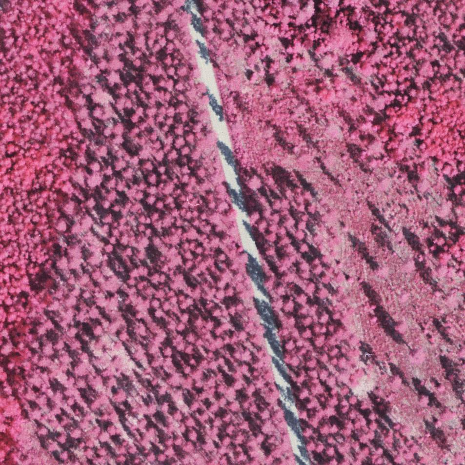
Kuva: Ortokuva samasta 200 x 200 m alueesta. Kuvamitt-ohjelmassa File | Create an orthoimage  -> *.RAW kuva, joka muutettu tässä JPG-muotoon. Aukot maaosumissa saavat selityksen: LK2 sijaitsee Lapinkankaalla, CT/VT-mäntykangasta. Vasemmalla näkyy nuorta mänty-hieskoivumetsää puolukkaturvekankaalla. Lisäksi kuvalla näkyy siemenpuuasentoon hakattu kuvio, jossa yksittäisten siemenpuiden latvukset ovat estäneet lidar-pulssin pääsyn maanpinnalle. A 200 by 200 m orthoimage of the same area was produced uinsg KUVAMITT's functionality (File | Create an orthoimage) which produces a raw-image that was converted into a JPG-file here. The gaps of ground points get an explanation: plot LK2 is situated in the Lapinkangas glacial delta which is a barren site dominated by pine. On the left (west) a young pine-pubescent birch stand on drained peatland is seen. The ground hits are less frequent there (cf. the map above). On the right there is a sparse seed tree stand. The gaps caused by individual crowns are seen in the map.

---

3) Kokeillaan yksinkertaista gradienttipohjaista menetelmää lidar-DTM estimoimiseksi ja raportoidaan sen tarkkuus muutamissa kohteissa (Gradienttipohjainen DTM:n suodatus lidar-pisteistä; D:\MINV12\ DTM_Filter\). Try out a simple gradient based mothod for estimating a DTM from unclassified lidar points. Study the accuracy in some target areas of your interest. Use the VB-program DTM_Filter.

Tehdään ohjelmilla D:\MINV12\ DTM_Filter\ ja D:\MINV12\DELANAY\ TIN-muotoinen DTM-malli, joka luetaan KUVAMITT-ohjelmaan. KUVAMITT-ohjelmaan joko luetaan tai mitataan joitakin maapisteitä (min 20) ja testataan tehdyn TIN-muotoisen DTM:n tarkkuus. Kohteen saa valita itse. Make a TIN-DTM using programs D:\MINV12\ DTM_Filter\ ja D:\MINV12\DELANAY\  and read it to KUVAMITT-program for the tests. You can either import a minimum of 20 reference points to KUVAMITT or measure them photogrammetrically.

Valitsin kohteeksi muistokuusikon (puutiedosto mk_treest.txt) I chose Muistokuusikko (mk_trees.txt observation file) as my target.

Tein DTM_filter ohjelmalla 300x300 m kokoisen suodatuksen muistokuusikon ympäristöstä ja ajoin ko. pistejoukosta DELANAY-ohjelmalla TIN-mallin eli *.nod ja *.tri tiedostot. KUVAMITT-ohjelmaa luin HydeLidarDTM- maastomallin (rasteri) sekä toiseksi maastomalliksi TIN-mallina tekemäni nod- ja tri-tiedostot. With DTM_Filter I created a TIN-DTM 300 by 300 m in area around Muistokuusikko and Hyytiälä forest station (see figures below). The TIN consists of a *.nod and a *.tri -file (compatible with Trinet software), which together with the raster-DTM by TerraModeler were imported to KUVAMITT for analysis.

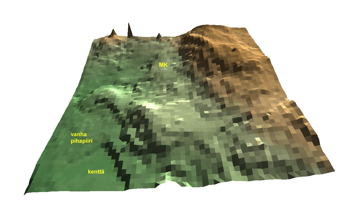
Kuva: Trinet ohjelmalla visualisoitu TIN muistokuusikon ja Hyytiälän metsäaseman pihapiirin alueelta (kts. www.pixtopo.com, "syö" samoja *.nod ja *.tri tiedostoja kuin KUVAMITT) Visualization of the TIN DTM created using the gradient based method. View from the south to Hyytiälä. See aerial view below. Muistokuusikko test stand in marked with "MK". Visualization with Trinet-software, see www.pixtopo.com)

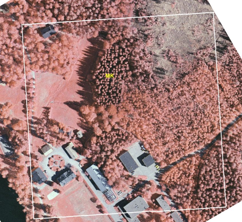
Kuva: Saman TIN-mallin rajaus ilmakuvalla. The 300 by 300 m coverage of the DTM seen an aerial view from 1997.

Muokkasin aliohjelmaa (Plot_Field_Plot_Data_Click()), jolla projisoidaan latvoja kuville se. kullekin puulle (x,y) pyydettiin TIN-korkeus ja Rasterimallin korkeus. Korkeuksien ero vaaitettuun puun korkeuteen tulostettiin ASCII-tiedostoon:
I altered the subroutine Plot_Field_Plot_Data_Click() that is used for projecting XYZ-data in aerial views in KUVAMITT, such that for each tree in position XY, the elevation was computed from both the raster and the TIN DTMs. The difference between the reference elevation was printed into an ASCII-file:
 
Rem READ record by record
Close (2)
Open "c:\data\MK_DTM_TEST.txt" For Output As 2
Dim MinZButt As Double, MaxZButt As Double
MinZButt = 1000
MaxZButt = 0
...
 z_butt = z - TreeHeight
 z_butt_raster = getheight(x, y)
 z_butt_TIN = getTINheight(x, y, CLng(0))
 
 Print #2, Format$(x, "#.00"), Format$(y, "#.00"), Format$(z_butt - z_butt_raster, "#.00"), Format$(z_butt - z_butt_TIN, "#.00")

ASCII-tiedostoon menivät 267 puun (pisteen) tiedot / This produced the resdiduals for the 267 trees in the stand
2515309.02    6859999.59    .21           .41
2515307.91    6860014.88    .39          -.38
2515309.83    6860018.80    .23          -.76
2515313.01    6860020.26   -.04           .02
2515306.00    6860023.27   -.25          -.21
2515306.34    6860023.56   -.07          -.08
2515312.26    6860023.23   -.30          -.43
2515314.98    6860029.48   -.17          .10
...

Kuva: Puukartta eli XY-testipisteet.Tree map of Muistokuusikko.

TIN-virheiden (erotusten) RMSE oli 0.43 m, keskiarvo 0.33 m ja hajonta 0.27 m, eli malli antaa keskimäärin 33 cm liian alhaisia korkeuksia. The differences had an RMSE of 0.43 m, a mean of +0.33 m and a STDEV of 0.27 m, i.e. the TIN gives elevations below the true ground.

Kuva: Terra-ohjelmistolla tuotetun rasteri-muotoisen mallin virheiden ja DTM-filter ohjelmalla tuotetun TIN-mallin virheiden yhteisjakauma muistokuusikossa (MK-trees.txt) The joint distribution of the errors by the TerraModeler-DTM (x) and gradient-based DTM (y). Virheiden yhteisjakauma osoittaa, että virheet ovat jossakin määrin korreloituneita; tämän voi tosin aiheuttaa myös virheet referenssidatassa; nehän (testipisteet) ovat samat molemmille. Kumpikin malli tuottaa liian maanpinnan liian alhaalle. The correlation may indicate that the reference data has errors.Both DTMs produce elevations below the true surface.


Kuva: TIN-mallin (Gradienttimenetelmällä tehdyn DTM:n) virheet Muistokuusikossa. TIN-malli on tuottanut pääsääntöisesti N60-korkeuksia "tosimaanpinnan alta"; maasto nousee alueella lounaasta-koilliseen. The errors of the gradient-based DTM in Muistokuusikko. The true elevation is from 152 to 161 m and there is a slope  from SW to NE.

---

4) Tutkitaan lidar DTM:n tarkkuutta taimikoissa tekemällä referenssimittaukset "taannehtivasti ja metsänhoitajalle sopivalla arvolla" wanhoilta ilmakuvilta. Study the accuracy of the (un-edited) Terramodeler DTM in young stands "retrospectively in a manner fit for the status of a forester" using old aerail photographs. Ryhmä mittaa 200 hajapistettä kuviolta (valinta opiskelijanumeron viimeiseen numeroon perustuen), joissa 2004 keilattaessa oli taimikko, mutta tarkoilla ilmakuvilla 1985–2002(4) tuore aukko. Alle on listattu kuvioiden keskipisteitä, arvioitu avohakkuuvuosi sekä ilmakuvat, joita tulisi käyttää.. The group should measure a total of 200 reference points from a forest compartment (selection based on student number), where, in 2004, when the lidar was done, the vegetation represented that of a young stand. There are large scale photography from 1985-2002 in which the stand is seen as a clear cut. See the list of compartments, center coordinates, assessed time of clear cut and the available images to be used.

Valitsin KUVION n:o 4 I chose compartment number 4


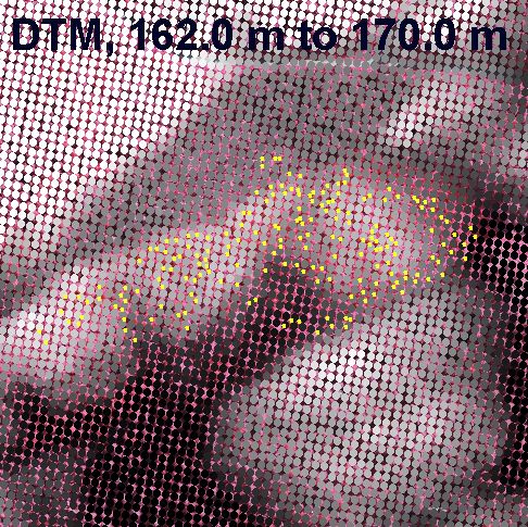
Kuva: Kuvion n:o 4 sisään mitatut 188 maapistettä (keltaiset, CTRL-P toiminto) projisoituna ilmakuvalle, johon on alle projisoitu harmaasävyllä DTM-pisteitä 5 metrin hilassa (TEST_DTM-valikkokomento, katso alempana), joiden harmaasävy on skaalattu lineaarisesti välille 162-170 m m.p.y. Pisteitä on mitattu noin 250 x 100 m alueelta 188 kpl. Topografialtaan alue on melko rauhallinen, minkä saattaa todeta anaglyfi-sterokuvasta vuodelta 1989 sekä yo. harmaasävykuvasta. Alueen lehtipuuston ja havupuutaimikon pituus vaihteli 3-7 m välillä 2004, kun lidarlento tehtiin. Kuviolle oli jätetty aliskasvosta 1989 (kts. anaglyfikuva), jonka johdosta puusto on hieman epätasaista 2004. The yealoow dots represent 188 reference points measured from an image pair taken in 1989 (1:5000). Dots in gray scale represent gournd points in a 5 m grid, with linear scaling of the grey tone between 162 m and 170 m a.s.l. The topography is fairly flat, which can be verified also from the anaglyph view from 1989 (below). The stand in 2004 consisted of 3-7 m high deciduous and conifer trees, with some larger trees (remnant from 1989, see anaglyph stereo view).

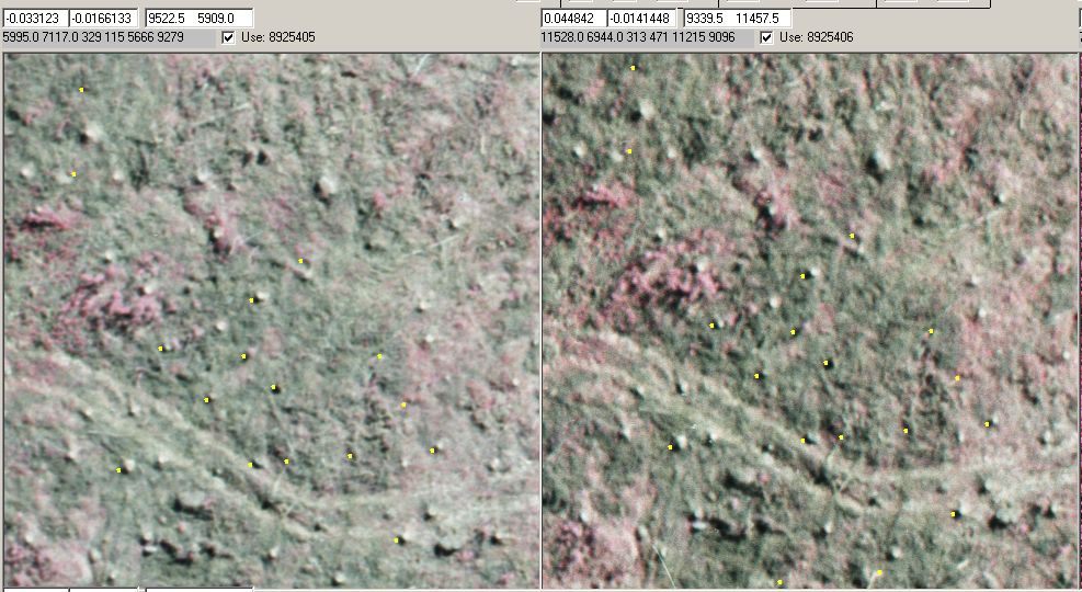
KUVA: Kuvio n:o 4 vuoden 1989 stereoparilla (1:5000, 15/23, 60-%), pikselikoko normalisoiduila kuvilla 45 um = 0.225 m. Mittamerkki (malli/näkymä) korkeudella 170 m. Anaglyph stereo view of 1989 with KUVAMITT, pixel of the normalized images is 22.5 cm.

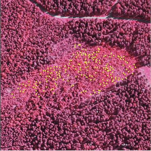
Kuva: Fotogrammetriset maapisteet kuvaparilla, joka alueelta oli hakkuuta seuranneelta kesältä. Pisteet mittasin varjoihin, mataliin kiviin tms. paljastumiin. Kantoja, joita olisi ollut käytettävissä runsaasti, en käytänyt, koska kannonkorkeus olisi pitänyt laskea havainnoista pois. An example of the reference points (a total of 188). The points are located in shadows, small stones, roots (+) etc. Stumps were avoided because it would have required substracting the butt heights (25-40 cm).

Kuva: LidarDTM-malli (TERRA-ohjelmistolla laskettu, raakahavainnoista 0.18 m nostettu) oli ko. kuviolla 20 cm "fotogrammetrisen maanpinnan alla". Jos yksittäisen foto-havainnon Z-tarkkuudeksi oletetaan 15 cm, saadaan keskiarvojen erotuksen (harha) keskivirheeksi 0.15 m / sqrt(188) = 0.011 m eli "harha on tilastollisesti merkitsevä". Näin ei tietenkään voida sanoa, koska emme voi olla 100 % varmoja siitä, ovatko foto-havainnot harhattomia Z:n suhteen eli antaako kuvapari (ja havaintomme) odotusarvoltaan oikeita N60-korkeuksia. Voi olla, että mittasin huomaamattani "kuoppia" tai "kumpuja", eikä niinollen maanpinta kaikkialla saanut samaa mahdollisuutta päätyä foto-mittaukseen. Samoin kuvaparin 8925405 ja 8925406 orientointi voi olla syst. väärin, jolloin kuvilta eteenpäinleikkauksena saadut XYZ-ratkaisut ovat siirtyneet/kiertyneet/vääntyneet.  The photogrammetric observations from 1989 were an average of 20 cm below the lidar DTM of 2004. Assuming that an indivial photo-observation has an accuracy of 15 cm, the difference of +0.20 m is "statistically significant", becuse with 188 observations the standrd error of the mean is 1 cm. There is of course no reason to present such claims, because the photo-observations cannot be quaranteed to be free from systematic errors (subjective selection of points, orientation of imaes).

Kuva: Karttakuva (MS-EXCEL, BUBBLE) erotuksista.  Seuraava vaihe analyyseissä olisi tutkia, selittävätkö 2004 ilmakuvilla näkyvä kasvillisuus residuaaleja tai topografian ominaisuudet. Virheet vaikuttaisivat lievästi korreloituneilta: "naapuri ennustaa naapuria". Tämä voi johtua siitä, että TERRA:lla maapisteitä luokiteltaessa maapistejoukko on jänyt harvaksi, jolloin välivaiheena syntynyt TIN-verkko oli harva, ja siis kolmiot (tasopinnat) laaja-alaisia. A map of the DTM errors obtained using the retrospective photogrammetric observations as reference. The next step would be to analyze the vegetation in 2004 (during the lidar, there is available imagery), and to study if the properties of the vegetation explain the errors in any way. One hypothesis is that TerraModeler would easily classify low, dense vegetation into ground points, thus lifting the DTM in places (unfilled dots in the map). The errors seem to have slight positive spatial correlation, i.e. "neighboring points predict eachother"..   

(Code for generating gray-level  maps (superimposed on the aerial views) of surface models in KUVAMITT)
Private Sub Test_DEM_Click()

Dim X_test As Double, Y_test As Double, Z_test As Double, k As Long, l As Long
Dim p_x As Double, p_y As Double

Dim MinDTM As Double, MinCHM As Double, Z_CHM As Double, DimMaxnSM As Double

MinDTM = 162: MaxDTM = 170  ' Scaling of grayscale values, between
MinCHM = 150: MaxCHM = 190  '   "           "                  "
MaxnDSM = 25                ' Scaling from 0 to MaxnDSM
Dim DemoCase As Long
DemoCase = 1 ' 1 = DTM-demo, 2 = DSM-demo, 3 = nDSM-demo

 If SolutionExists = True Then
   For k = -50 To 50
    For l = -50 To 50
     X_test = X_sol + k * 5
     Y_test = Y_sol + l * 5
     Select Case DemoCase
      Case 1 ' DTM
      Z_test = getheight(X_test, Y_test)
      Case 2 ' DSM
      Z_test = getCHMheight(X_test, Y_test)
      Case 3 ' nDSM / CHM
      Z_test = getheight(X_test, Y_test)
      Z_CHM = getCHMheight(X_test, Y_test)
      Z_ero = Z_CHM - Z_test
     End Select
   
  For i = 0 To NumOfImages - 1
   Call r_transform_ground_to_pixel(i, X_test, Y_test, Z_test, p_x, p_y)
  
     If Z_test > 0 Then
     Form1.Picture1(i).DrawWidth = win_info(i).pan_x * 30 + 1
     Select Case DemoCase
      Case 1
      Apu_z = 255 - (255 - (Z_test - MinDTM) * 255 / (MaxDTM - MinDTM)) ' DTM
      Case 2
      Apu_z = 255 - (255 - (Z_test - MinCHM) * 255 / (MaxCHM - MinCHM)) ' DSM
      Case 3
      Apu_z = 255 - (255 - (Z_ero - 0) * (255 / MaxnDSM))     ' nDSM CHM Scaling 0...25.5 m
     End Select
    
     If Apu_z < 0 Then Apu_z = 0
     If Apu_z > 255 Then Apu_z = 255
     Select Case DemoCase
     Case 1, 2
      Form1.Picture1(i).PSet ((p_x - (image_info(i).o_col + win_info(i).win_o_col)) * win_info(i).pan_x - 1, ((image_info(i).Height - 1) - p_y - (image_info(i).o_row + win_info(i).win_o_row)) * win_info(i).pan_y - 1), RGB(Apu_z, Apu_z, Apu_z)
     Case 3
      If Z_CHM > 10 Then
       Form1.Picture1(i).PSet ((p_x - (image_info(i).o_col + win_info(i).win_o_col)) * win_info(i).pan_x - 1, ((image_info(i).Height - 1) - p_y - (image_info(i).o_row + win_info(i).win_o_row)) * win_info(i).pan_y - 1), RGB(Apu_z, Apu_z, Apu_z)
      End If
      End Select
      Form1.Picture1(i).DrawWidth = 1
     End If
    Next i
   Next l
 Next k
  
 End If

   For i = 0 To NumOfImages - 1
    Picture1(i).CurrentX = 10
    Picture1(i).CurrentY = 10
    Picture1(i).Font = Arial
    Picture1(i).FontSize = 30
    Picture1(i).FontBold = True
    Picture1(i).ForeColor = RGB(2, 5, 40)
  
   Select Case DemoCase
    Case 1
    Picture1(i).Print "DTM, " & Format$(MinDTM, "#.0 m"); " to " & Format$(MaxDTM, "#.0 m")
    Case 2
    Picture1(i).Print "DSM, " & Format$(MinCHM, "#.0 m"); " to " & Format$(MaxCHM, "#.0 m")
    Case 3
    Picture1(i).Print "nDSM, " & Format$(CDbl(0), "#.0 m"); " to " & Format$(MaxnDSM, "#.0 m")

   End Select
   
   Next i


End Sub

---

5) Tehdään kokeita siitä, miten DTM-virheet näkyvät yksittäisten puiden d13- ja tilavuusestimaateissa, kun puulle mitataan pituus latvapisteen ja maanpinnan korkeuden erona, latvuksen leveys sekä puulaji. Experiment with DTM-errors; see how they affect the allometric estimates of single tree dbh and volume in STRS when a tree measured from the air for crown width, tree height and species, and these measurents are plugged into allometric equations.

Ryhmä konstruoi yksinkertaisen simulaattorin, jossa tehdään Gaussisia virheitä latvuksen leveyden mittauksessa, pituuden mittauksessa ja puulajin tunnistamisessa. Yhtälöt, joilla d13 ennustetaan muuttujista (puulaji, pituus, latvuksen leveys) saadaan teoksesta Kalliovirta ja Tokola (2005). Tilavuusyhtälöt, joilla rungon tilavuus ennustetaan muuttujista (puulaji, d13 ja pituus) saadaan Laasasenaho (1982) julkaisusta. The group constructs a simple Monte Carlo -type simulator that performs STRS, i.e. trees are measured for crown width, species and height and estimated for dbh (Kalliota and Tokola 2005) and volume (Laasasenaho 1982). Gaussian additive, uncorrelated error terms are used for simulating measurement (and model) errors.

Datana voi käyttää jotain D:\PUUDATA\ :n tiedostoista. Latvuksen leveyden "maastomitattu arvo", joka puuttuu ko. tiedostoista, lasketaan kääntämällä malli d13 = (puulaji, pituus, latvuksen leveys), vaikka regressioyhtälöiden kääntäminen ei tuotakaan "oikeita arvoja". Excel ohjelmassa Gaussisia virheitä voi tuottaa NORMINV() -funktiolla. The data files in D:\MINV12\PUUDATA\ are available, but these files lack the true crown width observations/values. Invert the dbh-models for "true" crown width. In excel, use NORMIN()-funkction for creating Gaussian error terms using the inverse distribution function metdod (Input evenly distributed probability - Output Gaussian deviates with appropriate expectance and variance),

KUVA:  Esimerkki simulaattorista, joka operoi Muistokuusikon 267 puulla, olettaen ne kaikki kuusiksi. Simulaattoriin on "ohjelmoitu" latvuksen leveyden (dcrm) ja puun pituuden (h) mittaus sekä allometrinen  rinnankorkeusläpimitan (d13) ja tilavuuden laskenta (v) malleilla. Allometriseen malliin lisätään suhteellinen Gaussinen 0-odotusarvoinen virhe ("allometrinen-kohina-%"). Oikeisiin pituuksiin lisätään epsilon ~N(odotusarvo,Hajonta^2) sekä latvuksen läpimittaan epsilon~N(Odotusarvo,Hajonta^2). Virheet eivät korreloi, eli mittaukset ovat riippumattomia. Tilavuusyhtälöihin ei lisätä mallivirhettä, joka olisi noin 8-10 %, ja joka melko varmasti korreloisi d13 = f (sp, dcrm, h) -mallin virheiden kanssa (tätä asiaa ei kukaan ole tutkinut). Esimerkissä mittaukset ovat virheettömiä, mutta allometrinen kohina on mukana: Tällöin yksittäisen puun d13 saadaan 7.8 % RMSE-tarkkuudella ja tilavuus 13.2 % RMSE-tarkkuudella. Kokonaistilavuus tulisi alirvioiduksi 0.5 %. An example simulator in EXCEL; that operates with the 267 trees of Muistokuusikko in Hyytiälä, assuming that all trees are Norway spruces. No species recognition process is included, i.e. the species is obtained free from errors. Includes processes which are affected by Gaussian additive errors: 1) measurement of crown width (dcrm) , 2) measurement of tree height, and 3) allometric estimation of dbh. The error of the volume equations is not included, since it wold most likely correlate (positively? negatively? no studies on this) with dbh = f( sp, dcrm, height) -models. IN the example shown, only the 8% "allometric Gaussian noise" in the dbh models is counted for: RMSE of dbh is 7.8 % and RMSE of volume 13.2 %. This is the maximal accuracy that can be expected for single trees with error-free measurements.


Kuva: Mittauksiin on lisätty harhattomia Gaussisia virheitä. Pituuden hajonta on 0.5 m ja latvuksen läpimitan 0.5 m. Nyt yksittäisen puun RMSE-tarkkuus on 10.8 % d13 ja 20.5 % tilavuudelle. This simulation has random measurement errors for dcrm and height. The RMSE of dbh is 10.8 % and RMSE of volume 20.5 %.


Kuva: Nyt dcrm-mittaukset tuottavat 50 cm aliarvioita 50 cm hajonnalla (hajonta tehty heteroskedastiseksi, jottei pienillä puilla tulisi negatiivisia latvuksia), piituuksiin tulee 30 cm liikaa, kun DTM antaa liian alhaisia korkeuksia (meidän tilanne) ja pituuksien hajonta on 0.7 m. => d13 aliarvioituvat 3%, tilavuudet aliarvioituvat 3.5 %. Systemaattiset mittausvirheet osin kompensoivat toisian.A simulation in which crown widths are underestimated and tree heights overestimated (DTM gives too low elevations, our case). This results in an underestimation of the total volume by 3.5%. Single tree dbh and volumes are also positively biased (underestimated)

Kuva: Harhaisten pituus- ja drcm-mittausten johdosta d13-h yhteisjakauma "liikahti vasemmalle ja ylös" ja sekottui d13-suunnassa allometrisen kohinan takia. (vrt. yo. kuvan simulaatio). Measurement and model errors are seen in the dbh-h distribution. Red dots represent the simulated cases and green dots are the "true values".