Erikoisharjoitus II  Luennoitsijan esimerkki Special assignment II, lecturer's example

Valitsin testimetsää Kuivajärven luonnonhoitometsästä läheltä pistettä (2514865, 6860960, 192). Ilmakuvilta mitatut puut ovat ko. alueella pitkiä. KUVAMITT-ohjelmalla, käyttäen hyväksi lidar-DTM (HyderLidarDTM.hdr) sain puiden pituuksiksi pituuksiksi 24-32 m. Latvusten leveys vaihteli välillä 2-7 m. I selected a test site in the Kuivajärvi old growth around the point (2514865, 6860960, 192). Using the photogrammetric observations and the lidarDTM I estimated that tree heigts range from 15-32 m and the crown widths from 3 to 7 m (see aerial view below) .


Kuva: Annetun pisteen ympäriltä ilmakuvalle 0440302 projisoidut  lidar-pisteet. Kohdealue jää kahden risteävän lidar linjan (strip) alle, skannauskulmien ollessa noin 10-13^o ja ± 1^o. Test area seen in aerial image 0440302 with lidar points superimposed. The gery level indicates elevation with a linear scaling between 185 and 215 m. The area is under two lidar strips (perpendicular) with scan angles from 10 to 13 degrees and ± 1 degree.

Yo. kuvassa lidarpisteiden, first ja last, harmaasävy skaalattiin välille Z = (185...227 m) » (0...255) ao. koodiriveillä osiossa. Code changes in KUVAMITT for producing the figure above:
Aliohjelma, jolla kuva tuotettiin: Private Sub plot_als_bin_file_Click()

      pu_z = 255 - (185 - LP.Zs) * 6
      If pu_z > 255 Then pu_z = 255
      If pu_z < 0 Then pu_z = 0
      Apu_z = pu_z
      Form1.Picture1(i).DrawWidth = 3
      Call r_transform_ground_to_pixel(i, LP.Xs, LP.Ys, CDbl(LP.Zs), p_x, p_y)
      Form1.Picture1(i).PSet ((p_x ....litania puuttuu........ - 1), RGB(Apu_z, Apu_z, Apu_z)     
 
If LP.Zf > 10 Then
      pu_z = 255 - (185 - LP.Zf) * 6
      If pu_z > 255 Then pu_z = 255
      If pu_z < 0 Then pu_z = 0
      Apu_z = pu_z
      Call r_transform_ground_to_pixel(i, LP.Xf, LP.Yf, CDbl(LP.Zf), p_x, p_y)
      Form1.Picture1(i).PSet ((p_x ....litania puuttuu........ - 1), RGB(Apu_z, Apu_z, Apu_z) 
End If

Lidar pisteet tiedostoon Lidar points into an ASCII-file

Seuraavaksi kirjoitin ko. alueen pisteet ASCII tiedostoon. Keskipiste on lähellä "KKJ-hehtaarin" keskipistettä; otin koko hehtaarin pisteet talteen rajaamalla 3D pisteen (fotogrammetrinen ratkaisu) ympärille 150 x 150 m alueen ao. lauseilla Plot_als_bin_file_Click() -aliohjelmassa: As the next step I had the lidar points written into an ASCII-file. Following two lines were altered in the Plot_als_bin_file_Click() -subroutine. Recall that (X_sol, Y_sol, Z_sol) is the 3D photogrammetric point solution that can be set or measured from the images.

If Abs(LP.Xs - X_sol) < 75.5 And Abs(LP.Ys - Y_sol) < 75.5 And Abs(LP.Xf - X_sol) < 75.5 And Abs(LP.Yf - Y_sol) < 75.5 Then
   If Abs(LP.Zs - Z_sol) < 100 Then

Saman aliohjelman alkuun lisäsin lauseen, jolla avattiin ASCII-tiedosto tulostusta varten In the same routine, a line of code was added for opening the ascii-fle for output.
Open "c:\data\lidar_pisteet_LH_metsa.txt" For Output As 6
Aliohjelmaan laitoin ennen For i = 0 to NumOfImages -lausetta rivin tulostusta varten; talteen menee koko pulssin sisältö, yhteensä 18 muuttujaa per pulssi: In the same routine, just before the statement For i = 0 NumOfImages, I added a line of code for printing the full contents of the lidar-pulse into the ascii-file.
Print #6, LP.GPS_time, LP.omega, LP.phi, LP.kappa, LP.Xl, LP.Yl, LP.Zl, LP.Scan_angle, LP.Xf, LP.Yf, LP.Zf, LP.Intf, LP.Rangef, LP.Xs, LP.Ys, LP.Zs, LP.Ints, LP.Rangel
Aliohjelman loppuun tarvitaan tiedoston sulkeva lause And finlly, in the end of the rouine I added a line of code that closes the ascii-file.
Close (6)


Kuva: Yhden hehtaarin first return -pisteet (LP.Xf, LP.Yf) tasossa. Skannauskulman vaikutus tulee esille pisteiden XY-jakaumassa. Huom! kuinka havaintoja on ko. hehtaarin ulkopuolelta - pulssi on "sijoitettu siihen hehtaariin", johon last return -piste osui! Lidar data covering one hectare (recall that the lidar data is stored in one hectare files, checkboard-style). First return pulses as an XY map. Data from the two strips is shown in different color and the effects of the scan angle ("oblique viewing") are seen in the two point patterns.

Referenssipuut Reference data

Mittasin 321 puuta ilmakuvilta pisteen (2514865, 6860960, 192) ympäristöstä; pyrkien paikantamaan kaikki kuvilla näkyvät puut. Mittaukset tein 04403 kuvilta, jotka on otettu 2 viikkoa ennen lidar-dataa. Mittasin yhtenäisen alueen, joskaan en koko hehtaaria. I positioned by manual multiple image-matching, using three images from flight 04403, a total 321treetops in the neighborhood of the center point. A whole/unbroken area was covered, however not the full one hecrate area for which the lidar data is.


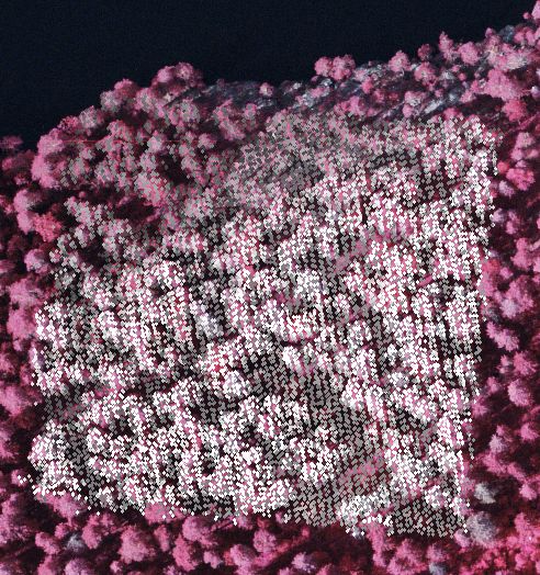
Kuva: referenssiaineistoksi (latvapisteet) mitatut pisteet projisoituna ilmakuvalle 0440302. Maasto laskee kohti järven rantaa kuvan ylälaidassa. Järven pinta on noin 141 m m.p.y (N60) ja maaston korkeus nousee 165 m. Rannassa (ylh. oik) on myös jyrkkiä rantakallioita, joilla kasvaa harvaa mäntymetsää. The reference tree tops seen in the aerial image 0440302. The terraiin slopes towards the lake seen in the upper part of the photo. The lake is ca. 141 m a.s.l and the terrain raises up to 165 m. There are steep areas near the lake (cliffs, rocky terrain, sparsely old pine trees).


Kuva: Referenssipuut (312) karttana. The reference treetop on an XY map.

Matlab-pintamallit

Muokkasin Juhan do_DTM_CHM.m ja find_trees.m Matlab-tiedostoja (kts alla) ja yhdistin ne yhdeksi komentotiedostoksi, joka lukee hehtaarin lidar-pulssit (pisteet), muodostaa DTM-, DSM-, ja CHM-pinnat sekä etsii puiden latvoja CHM:n lokaaleina maksimeina. DTM kirjoitetaan binääriseksi tiedostoksi, jonkA voi lukea KUVAMITT-ohjelmaan. Binääriselle DTM:lle tulostetaan "kaveriksi" ASCII HDR-tiedosto. Saadut latvat kirjoitetaan ASCII-tiedostoksi (puutiedosto), jonka voi lukea KUVAMITT-ohjelmaa ja projisoida latvat. Lopuksi rutiini tarkistaa yksinkertaisella menetelmällä, mitkä puut tulivat löydetyiksi sekä piirtää tasossa ja 3D kyseisille puille paikannusvirhevektorit (quiver-funktio). I edited Juha's Matlab sample m-files do_DTM_CHM.m and find_trees.m and combined them into one m-file. In it, the lidar data is read, surfaces: DTM, DSM and CHM are formed, and tree tops are found based on the assumption that they are represented by local maxima of the CHM. The DTM is stored into a binary file compatible with KUVAMITT (with hdr-file). The treetops are stored into an ASCII file, which is compatible with KUVAMITT, and KUVAMITT can be used for projecting the points on aerial images for visual check. Finally, the m-file performs a crude evaluation and produces information about omission and commission errors and positioning accuracy. Quiver-function is used for displaying results in 2D and 3D.



Kuva: osa(), "minimipinta", jossa reiät (puuttuvat havainnnot) ovat tasolla 500 m. Visualization of array osa(), which has no-data values at 500 m a.s.l.


Kuva: Maastomalli: dtm(), 21x21 ja 11x11 naapurustoilla suodatettu versio. Visualization of array dtm().

Kuva: dsm(); maksimeista suodatettu (griddata-funktio) pintamalli. Array dsm(), filtered with griddata() -function.

kuva: chm() = dsm()-dtm(). Normalisoituu pintamalli = latvuston korkeusmalli. Normalized DSM i.e. CHM.


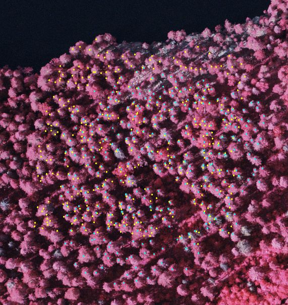
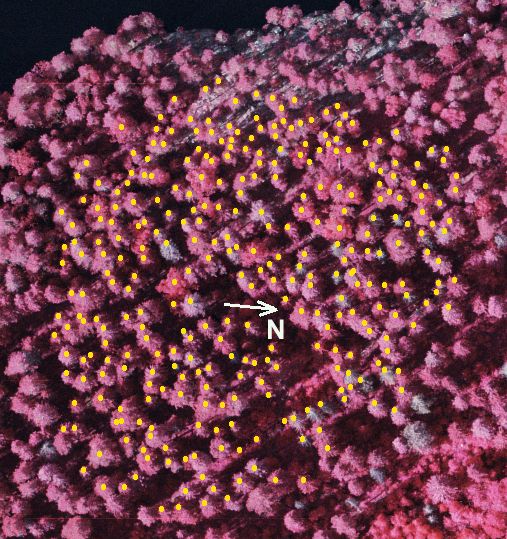
Kuva: Lidar-CHM :n lokaaleista maksimeista saadut latvapisteet projisoituna (CTRL-Q -toiminto KUVAMITT-ohjelmassa)  ilmakuvalle (keltaiset) sekä referenssipuut (siniset) (modifioitu CTRL-P-toiminto). The lidar CHM maxima superimposed in an aerial view (yellow dots) and the reference tre tops in blue.
.
Kun KUVAMITT-ohjelmaan oli luettuna lidarista TerraModeler -ohjelmalla konstruoitu DTM (HydeLidarDTM.hdr), oli puiden tyvien (eli Matlab-koodilla lasketun dtm-pinnan) korkeustarkkuus RMSE-virheenä mitaten 0.46 m, olettaen, että Terralla laskettu
malli "on oikea".The Matlab dtm-values (for the "trees" found in the lidar data )  had an RMSE of 0.46 m when compared with the DTM obtained with TerraModeler (giving RMSE we must assume that the Terramodeler model is correct!)

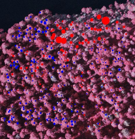
Kuva: Juhan koodilla tuotetun DTM:n ja TErraModeler-ohjelmalla lasketun HydeLidarDTM.Hdr erot (610 pistettä, h > 10 m). Punainen väri indikoi, että HydeLidarDTM.Hdr on korkeammalla. Suurin ero on -3.04 m. Matlab-koodi on "syönyt rinnettä". Differences between the matlab-dtm (modified Wack, as Juha called it) and the DTM produced with TerraModeler-software. 610 points (lidar trees). Largest difference is -3.04 m, the matlab-dtm underestimates elevation in the slopes ("it eats up the terrain"). Again, we do not know if the TerraModeler DTM is actually any better, because true reference is missing!

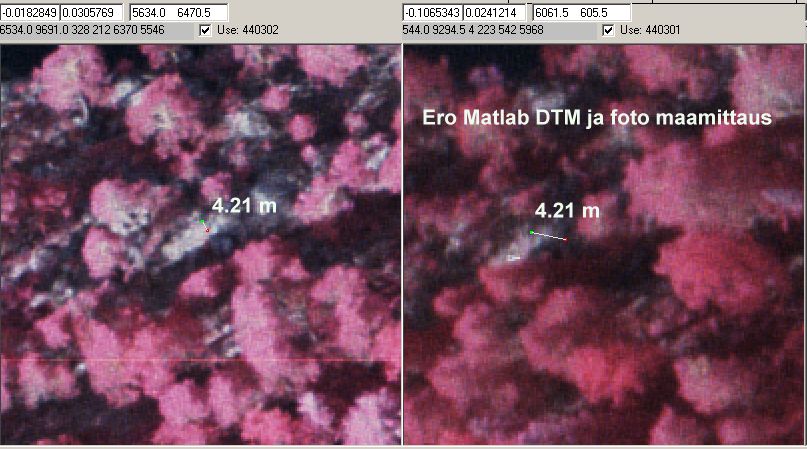
Kuva: Maanpinnan fotogrammetrisen korkeuden ja Matlab-DTM:n ero oli 4.2 m rinteessä. Samassa paikassa ero TerraModeler-malliin oli 1.8 m eli ei sekään vaikuta huipputarkalta. Inplaces the terrain is visible in aerial views. Here, the matlab dtm is off by 4.21 m in comparison to photogrammetric Z. For the same point, the TerraModeler-DTM was off by 1.8 m, so if the the photogrammetric observation really applies ground, neither of the DTMs is quite correct.

Kuva: Säteeltään 20-metrisen ympyräkoealan sisällä on referenssilatvoja (+), joille on löydetty lidar-CHM-maksimi. Sininen vektori osoittaa ko. pisteeseen. Kuvasta näkee, kuinka mätsäysalgoritmi sallii duplikaatit, eli samaan puuhun sallitaan useampi osuma. Lidar-osumat ovat tosilatvojen alta. The matlab-code displays the reference tree tops (+ signs) and "lidar-found trees" in 3D.  The blue vectors point to the lidar-tree tops which map to the particular tree. The matching algorithm allows for duplicates (vectors pointing to the same point), which is not very clever.