Introduction
Our 2006 LiDAR data set has an average density of 7 pulses per m2. Most of the pulses have only 1 return, i.e. an XYZ-point with associated intensity value. When the Dcrm of an individual tree is approximately 2-5 meters, we can assume that 22-137 pulses have "intersected" the crown surface area. If the scanning is from above (nadir), these values give a reasonable range of the number of possible hits in a crown. The 2006 LiDAR data set had a maximal off-nadir scanning angle of 14 degrees, which means that for conical crowns, for example, the values are slightly too high.
The ALTM 3100 sensor was operated from 800 m AGL. The beam divergence was 0.3 mrad, which means that the lidar pulse was 0.24 m wide (certain proportion of the pulse energy was within this cone). Any gaps in the crown that were wider than 0.25 m allowed the pulse to "move on". Any targets (reflectors) that were intersected by the laser pulse (cone of collimated light at 1064 nm, 3 m "long" pulse) produced an echo that was registered by the instrument. This is illustrated in Fig. 1 and 2.
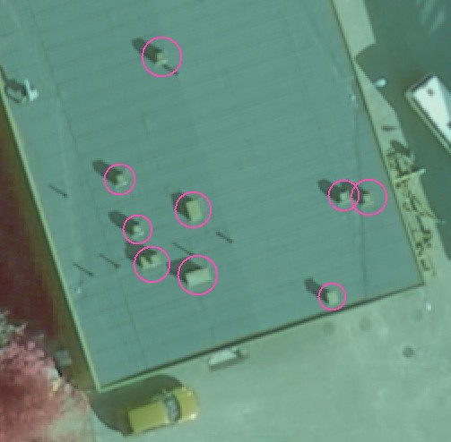
Fig. 1. The roof of a almost flat building (20 x 20 m seen). Nine 50-70-cm high chimneys are marked by the circles.
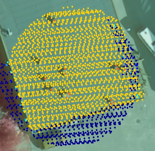
Fig. 2. The LiDAR "found" 8 of the 9 chimneys. Because of the rather small size of the objects - largest chimney is 0.7 x 1.2 m - the number of hits per target (1-3) does not well correlate with the actual size. Note also the slight (< 20 cm) mismatch between the image and LiDAR data.
The 6-8 pulse per m2 density limits the size of objects that can be detected (Fig 1-4).
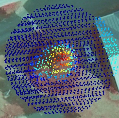
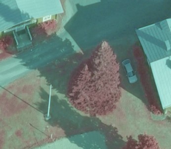
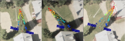
Fig. 4. The non-nadir image reveals that there
actually are two tops. The image here has GSD of 9 cm, which means
that the object is sampled for 123 pixels per m2.
Reconstruction of edges and other sharp changes in the structure of the object require a high sampling rate. For example, the position of the low-left corner of the roof in Figs 1 and 2 is accurately measured from images, but cannot be determined accurately using the lidar points seen in Fig 2. The corner will be round, if the the LiDAR data is used. On the other hand, the LiDAR data in Fig 2. can be used for the determination of the elevation of the roof or the terrain, which have very little texture in the images to support image-based 3D reconstruction. The second tree top in Figs 3 and 4 is easily missed because it so close to the bigger tree, but it is well seen in Fig 4, which has 123 samples per m2.
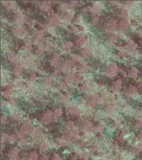
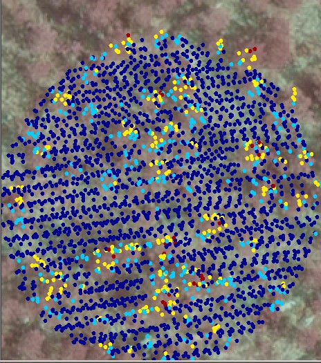
Trees in seedling stands are difficult to discern in the images and very high density of LiDAR would be required for STRS: in the order of 30-40 pulses per m2. Fig 5. illustrates how the 6-8 point density is insufficient for small trees.
Reconstruction of edges and other sharp changes in the structure of the object require a high sampling rate. For example, the position of the low-left corner of the roof in Figs 1 and 2 is accurately measured from images, but cannot be determined accurately using the lidar points seen in Fig 2. The corner will be round, if the the LiDAR data is used. On the other hand, the LiDAR data in Fig 2. can be used for the determination of the elevation of the roof or the terrain, which have very little texture in the images to support image-based 3D reconstruction. The second tree top in Figs 3 and 4 is easily missed because it so close to the bigger tree, but it is well seen in Fig 4, which has 123 samples per m2.
Trees in seedling stands are difficult to discern in the images and very high density of LiDAR would be required for STRS: in the order of 30-40 pulses per m2. Fig 5. illustrates how the 6-8 point density is insufficient for small trees.
Fig. 5. 20 x 20 m view to a sparse 10-yer
old seedling stand. The LiDAR points are HSV-coded between 0-4 m AGL. The
LiDAR point distribution is rather irregular, which means that "the effective
sampling density" is less than the nominal point density. The zigzag-pattern
of two strips is seen, and the two strips overlap leaving non-sampled gaps,
especially in the flight direction (vertical direction in the images).
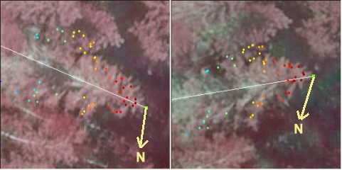
If the LiDAR pulses do not meet the apex of the crown, underestimation of tree height is unavoidable (Fig. 6). Also, for the measurement of Dcrm using LiDAR, observations of the very tips of branches are needed (Fig. 6 - 9).
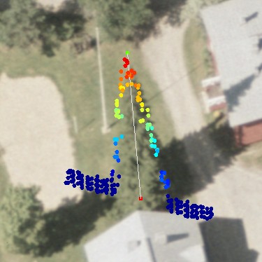
The siberian fir in Fig 6 has a very compact crown that reaches down to the ground. Fig 8. illustrates a 26-m spruce and a 20-meter high birch. The LiDAR points somewhat underestimate the extent / volume of the crown envelope seen in the images.
Back to index,
Next
Measuring Dcrm with Lidar and a parametric crown model
Crown model
Crowns are complex 3D objects, but we can try to model them using assumptions that simplify things. In object recognition, we can use a model-based strategy. In it, we use an implicit or an explicit model for the object to be detected. In template matching, it was possible to use explixit 3D geometric-optical crown models that were used for generating the template images, which were used for finding the trees. Copying the templates from the real images illustrates the use of an implicit object model. With LiDAR, we can use a simple model for the crown envelope, and try to measure the shape of crowns in the LiDAR data using the model as a starting point / approximation.
Our simple crown model assumes that the crown has an opaque smooth surface. To further simplify it, we can assume that branches at a certain height are all of equal lenght - i.e. the model is rotation symmetric. The crown has a certain depth. There is variation in crown lenght between tree species, and inside one stand, the density and site conditions affect how long the crowns are (self-pruning). If there would be a way to measure the height of the lowest living branches, it would be possible to set the depth of the crown as a free parameter to be solved from the LiDAR data. Such methods exist, but in the articles where they are tested, the LiDAR density has been around 30 pulses per m2 and the articles apply to mature stands.
In allometric modeling - dbh = f(sp, Dcrm, h) - the models assume that the crown width estimate is the maximum crown width. The maximum is low in young trees, but moves upward later. To start with a simple model, we can assume that the maximum is always at the 60 or 70 % relative height. This assumption is justified by the fact that we usually don't have many points that represent the lower parts of the crown, because of the oblique scanning. For example, in a 75-yr old dense spruce stand (Muistokuusikko in Hyytiälä), where heights are from 25 to 28 m, the height distribution of the LiDAR points was: < 5 m 42.5%; 5-10 m 1.7%; 10-15 m 4.0%; 15-20 m 18.7%; 20-25 m 27.4%; > 25 m 5.0%. The proportion of points between 5 and 15 meters was small, because there was no understorey and the height of the lowest living branches is apprx. 15 meters.
Fig. 10. If we know the position of the treetop,
we can treat LiDAR hits as observations of crown radius at a certain relative
height, r(hr).
If we know the treetop position, we have an estimate of height. If we know the species in addition to height, we can guess the size and shape of the crown envelope using our knowledge in allometry (Fig. 11):
Fig. 11. Basic crown models for a 22-m high
birch, pine and spruce. Values for a shape parameter (a2 in [1]
below) are given. The crown length is 40% for all species i.e. the crown extends
from the 100 % relative height down to the 60% relative height.
The crown surfaces in Fig 11 are curves of revolution
The crown surfaces in Fig 11 are curves of revolution
r(hx) = a1 × h ×
sin(hx)a2 + a3
[1]
h is the tree height. hx the (relative) height of interest. It must be scaled between (0..PI/2) to make the term sin(hx) scaled between (0..1). sin(hx) = 0 at the treetop and sin(hx)=1 at the lowest part of the crown, which can be for example the 60% relative height as in Fig 11. The term a1 gives a relation ship between tree height and maximum r. a3 is a constant term, which makes the top of the tree "flat" if it deviates from zero.
[1] is a non-linear function in the parameters a1, a2 and a3, which must be accounted for in their estimation using least square optimization.
Finding the LiDAR hits of a particular tree
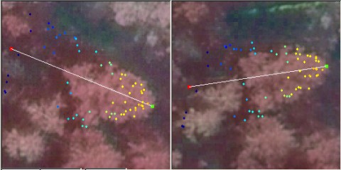
When the tree is open grown or has no neighbors, the LiDAR hits that "belong" to this tree are unambiguosly defined. It is easy to collect them, and if the treetop XYZ-position is known, the variables of [1] are easily computed. However, in closed canopies the situation is more complex (Fig 12). The canopy structure can make the use of LiDAR for STRS difficult, when branches of trees are interlaced: e.g. in young and dense spruce plantations. If we wish to use [1] and LiDAR points for the estimation of its three parameters, we must be able to collect the correct LiDAR points that have echoed from the crown of interest (Fig 12-15).
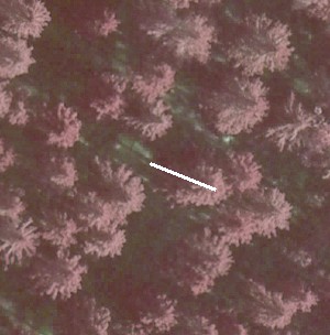
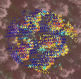
Fig. 13. The LiDAR-points that are within 3
m in XY from the treetop of the 25.5-m high spruce in Fig 12. The treetop
XYZ-position was measured using multi-scale TM in aerial images. The point
distribution show the crown shape of the first 5 meters down from the top
(down to 80% height). There are some points that have echoed from inside the
crown envelope (-6 m, 0.8 m) and (-8 m, 0.3 m). The point distribution
also suggests that the crown radius 10 meters down from the apex is somewhere
between 1.4 and 3 meters, which is 2.8-6 m in Dcrm. In a NFI data set, 25-m
high spruces have been measured Dcrm between 3 m and 7 m. Fig 12. shows that
the tree of interest has a neighbor that is some 3 meters away. It is obvious
that not all points are from our tree of interest.
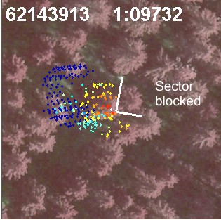
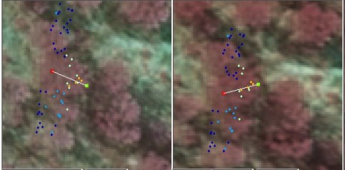
Fig. 14. If we know the treetop positions prior
to the estimation of the crown models, we know that there is a tree 3 m away
from the tree of interest. Here, a 90-degree wide sector has been determined
to filter the noise from the neighbor that is too close and which likely
has interlaced branches with our tree.
To get the correct set of LiDAR observations is subject to errors as Figs 11-15 illustrate. If we know the species, height, and the treetop 3D position for the tree-of-interest and its neighbors, we can do better. Knowing the species and height can be used for defining a range of expected Dcrm (maximum) and a basic crown shape (Fig 11). For example, spruce trees in NFI data of Finland, show a linear relationship between height [m] and Dcrm [m]:
Dcrm = (0.15 × h + 1.4) ×
Correction [2]
In very dense stands, the Dcrm is overestimated (Correction = 0.7) and in very sparse (grown) stands [2] underestimates the Dcrm (Correction = 1.25). I.e. there is considerable variation in the Dcrm/height ratio and actually we hope that it will be reflected in the dbh-estimation that follows as the last step of STRS - if we can measure Dcrm and height accurately, we have better estimation accuracy of dbh than with height alone.
When we look for the LiDAR points that belong to our tree - of - interest and fit a crown model to the data, it would be possible to start "carefully" from the top of the tree and to fit the crown model first there. Then move downwards and include mode LiDAR points to the set of observations and filter neighbors as illustrated in Figs 14-15.
Our implementation on MARV4/2 is simple and crude, however. In it, the height/Dcrm relationship [2] is taken into use with basic crown models [1]. The height and species information that are known defore crown fitting starts, define a basic crown model and LiDAR points inside the volume bounded by the basic model are used for the estimation of [1]. In other words, we have initial values for the parameters a1, a2 and a3 of [1] and change the size of the model using a "Correction" coefficient (c.f. [2]). Then we fit the data and get "better" estimates of a1, a2 and a3 of [1] (Fig 16).
Fig. 16. At the start, the crown model
[1] is an overestimation: start value of a1 sets the "scale", a2 sets the
initial shape and a3 defines how large is "the plateau" at the top. Least
square fit (crown modeling) with the LiDAR data is done iteratively since
[1] is non-linear. Here the RMSE of crown radius values is 0.31 m after the
final iteration. The last drawn model shows that a3 has a negative value at
the optimum, since the crown radius is zero some distance down from the top.
The RMSE of the fit is an indicator of the success. If it is large, it is possibly due to errors in the LiDAR data set - wrong observations have been used.
Notes
- In reality crowns are asymmetric (due to mechanical stress, shading). Crowns overlap in dense stands, which means that it is impossible to separate two crowns by one line between them.
- Least square fitting (see Fig 15) of the crown model [1] to the LiDAR data is non-optimal since it produces a surface that minimizes the positive and negative residuals (sum of their squares) of crown radius, and we know that our observations are by default biased, because LiDAR did not seek its way to the tips of branches.